
 Stephen Senn
Head, Methodology and Statistics Group,
Competence Center for Methodology and Statistics (CCMS),
Luxembourg
At a workshop on randomisation I attended recently I was depressed to hear what I regard as hackneyed untruths treated as if they were important objections. One of these is that of indefinitely many confounders. The argument goes that although randomisation may make it probable that some confounders are reasonably balanced between the arms, since there are indefinitely many of these, the chance that at least some are badly confounded is so great as to make the procedure useless.
This argument is wrong for several related reasons. The first is to do with the fact that the total effect of these indefinitely many confounders is bounded. This means that the argument put forward is analogously false to one in which it were claimed that the infinite series ½, ¼,⅛ …. did not sum to a limit because there were infinitely many terms. The fact is that the outcome value one wishes to analyse poses a limit on the possible influence of the covariates. Suppose that we were able to measure a number of covariates on a set of patients prior to randomisation (in fact this is usually not possible but that does not matter here). Now construct principle components, C1, C2… .. based on these covariates. We suppose that each of these predict to a greater or lesser extent the outcome, Y (say). In a linear model we could put coefficients on these components, k1, k2… (say). However one is not free to postulate anything at all by way of values for these coefficients, since it has to be the case for any set of m such coefficients that ![]() where V( ) indicates variance of. Thus variation in outcome bounds variation in prediction. This total variation in outcome has to be shared between the predictors and the more predictors you postulate there are, the less on average the influence per predictor.
where V( ) indicates variance of. Thus variation in outcome bounds variation in prediction. This total variation in outcome has to be shared between the predictors and the more predictors you postulate there are, the less on average the influence per predictor.
The second error is to ignore the fact that statistical inference does not proceed on the basis of signal alone but also on noise. It is the ratio of these that is important. If there are indefinitely many predictors then there is no reason to suppose that their influence on the variation between treatment groups will be bigger than their variation within groups and both of these are used to make the inference.
I can illustrate this by taking a famous data-set. These are the ‘Hills and Armitage enuresis data’(1). The data are from a cross-over trial so that each patient provides two measurements; one on treatment and one on placebo. This means that a huge number of factors are controlled for. For example it is sometimes claimed that there are 30,000 genes in the human genome. Thus 30,000 such potential factors (with various possible levels) are eliminated from consideration, since they do not differ between the patient when measured on placebo and the patient when measured on treatment. Of course there are many more such factors that do not differ: all life-history factors including what the patient ate every day from birth up to enrollment in the trial, all the social interactions the patient had during life to date, any chance infection the patient acquired at any point etc, etc. The only factors that can differ are transient ones during the trial, what are sometimes referred to as period level as opposed to patient level factors.
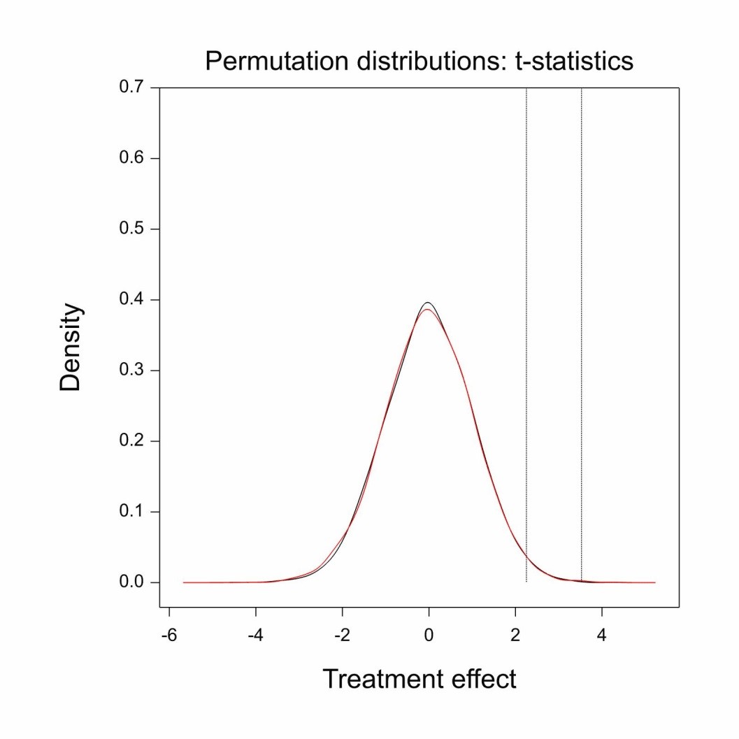
The figure below shows two randomisation analyses of the trial. One uses the true fact that the trial was a cross-over trial and pairs the results patient by patient, only randomly swapping which actual observed outcome in a pair was under treatment . The other pays no attention to pairs and randomly permutes the labels around only maintaining the total numbers under treatment and placebo.
What is plotted are the distributions of the t-statistics, the signal to noise ratios, and it can be seen that these are remarkably similar. Controlling for these thousands and thousands of factors has made no appreciable difference to the ratio because any effect they have on the numerator is reflected in the denominator. What changes, however, is where the actual observed t-statistic is placed compared to these permutation distributions. The t-statistic conditioning on patient as a factor is 3.53 (illustrated by the rightmost vertical dashed line) and the statistics not conditioning on patient is 2.25 (illustrated by the left-most line). This shows that if we realise that this is a cross-over trial and therefore that differences between patients can have no effect on the outcome, the observed difference is much more impressive.
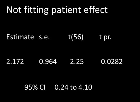
 This fact is reflected in the parametric analysis. In the table below, the left hand panel shows the analysis not putting patient in the model and the right hand one the analysis when patient is put in the model. On the LHS, the t-statistic is less impressive and so is the P-value than is the case on the RHS. The point estimate of 2.172 dry nights (the difference between treatment and placebo) is the same.
 |
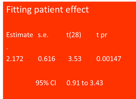 |
This brings me on to the third error of the ‘indefinitely many predictors’ criticism. Statistical statements are statements with uncertainty attached to them. The reason that the point estimate is the same for these two cases is that we did in fact run a cross-over trial. If we had run a parallel group trial instead with these patients, then it is unlikely that the treatment estimate delivered would have been 2.172 which it was for the cross-over. The enemy of randomisation may say this just shows how unreliable randomisation is. However, this overlooks the fact that the method of analysis delivers with it a measure of its reliability. The confidence interval for not fitting the patient effect is 0.24 to 4.10 and thus much wider than the interval of 0.91 to 3.43 when it is fitted.
In fact the former method has allowed for the fact that thousands and thousands of factors are not fitted. How does it do this? It does this by using the very simple trick of realising that these are only important to the extent that they affect the outcome and that variation in outcome can be measured easily within treatment groups. The theory developed by Fisher relates the extent to which the outcomes can vary between groups to the extent to which they vary within. Thus randomisation, and its associated analysis, makes an allowance for these indefinite factors.
In fact the situation is quite the opposite of what the critics of randomisation suppose. Randomisation theory does not rely on indefinitely many factors being balanced. On the contrary it relies on them not being balanced. If they were balanced then the standard analysis would be wrong. We can see this since in the case of this trial it is the RHS analysis controlling for the patient effect that is correct since the trial was actually run as a cross-over. It is the LHS analysis that is wrong. The wider confidence interval of the LHS analysis is making an allowance that is inappropriate. It is allowing for random differences between patients but such differences can have no effect on the result given the way the trial was run. Further discussion will be found in my paper ‘Seven myths of randomisation in clinical trials’(2).
References:
1. Hills M, Armitage P. The two-period cross-over clinical trial. Br J Clin Pharmacol. 1979; 8: 7-20.
2. Senn S. Seven myths of randomisation in clinical trials. Statistics in Medicine. 2012 Dec 17.
(See also on this blog: S. Senn’s July 9, 2012 post: Randomization, ratios and rationality: rescuing the randomized clinical trial from its critics.)


")


Stephen: Thanks so much for your interesting post. Your points clarifying the thorny issue of randomization and statistical inference are welcome (as they so often arise, especially in philosophy). So how would you say these points relate to all the efforts pre data to stratify, and post-data to check for homogeneity? In a discussion of one of the early studies on birth-control pills and clotting disorders (chapter 5 of EGEK), I noted the analyses carried out, post data, to ensure that the treated and control women were sufficiently homogenous with respect to the chance of a blood-clotting disorder, by a series of null hypothesis tests on age, number of pregnancies, income etc. No statistical significances were found. Are you saying it wouldn’t have mattered (for the validity of testing the effect of the pill on clotting disorders) if they had been found, but at most the accuracy or the like? In this connection, I’m not completely sure I get the point as to why RCTs depend on the group being imbalanced, in general.
Dr. Senn,
I read your paper on the seven myths and gained fresh perspective. I have a quibble, so naturally I’m going to go on and on about the part I disagree with, passing over the other unobjectionable (indeed, edifying) content in silence.
My quibble is in regard to your comments on Lindley. In my view, he has the right of it, and your criticism, while not wrong, is shallow; it takes little effort to answer it.
Rather than getting hung up on the word “haphazard”, let’s see what we can make of the question of whether the lady is “reasonably entitled to make the assumption of exchangeability”. Suppose that our experimental design scheme is to take the previous day’s horse racing program (without bookies’ odds) and construct a map from possible outcomes to the 70 possible tea experiment designs. We suppose that the lady in question is fully informed about the mapping, but, like us, does not know the races’ outcomes or the odds that were offered. We then go, find the race results, mix the tea, and have it sent out to her. Is she entitled to make the assumption of exchangeability?
It depends. Perhaps she is an aficionado of horse race betting; although the previous days’ results are unknown to her, she knows the horses and can set her own reasonably well-informed odds.
So we come up with another scheme. Instead of yesterday’s race results, we’ll come up with a mapping between the lengths of the reigns of the rulers of the Goryeo dynasty (from which modern-day Korea gets its name) and the 70 possible designs. That should be sufficiently haphazard, no?
But what if she’s an historian specializing in the postclassical Far East? Let’s instead use the digits of the permitivity of free space. But perhaps she’s a physicist, so let’s use some far digits of pi. But maybe she’s a mnemonist! All right, fine, let’s just do the randomized design. As long as she isn’t psychic…
But it turns out she’s no gambler, historian, physicist, nor mnemonist (and not psychic) — she was a statistician all along. For her, race horses are exchangeable; she doesn’t know the Silla kingdom from the Joseon dynasty; she has no need of the vacuum permitivity constant in her work, and she’s too sensible to spend time memorizing digits of pi. Any of our schemes would have supplied the necessary conditions. Randomization’s virtue, as you note in the paper, is that it’s a particularly cheap and robust way making sure there’s no extraneous information being used to make the predictions.
Corey, I always start this argument from the other end. For me a randomised allocation is one in which each of the 70 sequences are equally likely. Now Lindley says that other schemes (such as, presumable, the ones you describe) are acceptable even though strictly speaking all sequences are not equally likely. However, to be fully Bayesian, in that case he has to model the probability with which she will guess the scheme. It seems to me that all you are doing is putting a very small probability on guessing.
This is what I have referred to elsewhere as ‘the argument from the stupidity of others’. It is the implicit argument that the German enigma coders made in the Second World War and the fact that it turned out to be wrong was why Bletchley Park were able to break the code.
More generally, I have found that (some) Bayesians assume too lightly that all is well if you don’t randomise. I am not accusing you of this and you described some schemes in detail, which is more than I usually get. However, look at Urbach’s proposal for allocation of patients to treatment referred to in my Seven Myths paper if you want an example of how things can go wrong.
SJS: I guess the point Lindley was making that I’m trying to highlight is that the key question is always: “what information (other than taste) does the lady tasting tea have that can help her predict the mixing order (i.e., the information breaks exchangeability)?” To see this, suppose we divide the interval [0, 1] into 70 subintervals of equal length, pick a mapping specifying one design per subinterval, generate a uniform random deviate, and so on. Everything’s hunky-dory, right? Well, unfortunately, somehow the protagonist got ahold of the first digit of our input, so she was able to rule out 7 designs without even tasting the tea. The mere fact randomized allocation wasn’t good enough. (I’m assuming that the mapping from the uniform random variable to the chosen design is known to the protagonist, which is an equivalent setup to my set of examples above).
The example of this comment plus the examples of my previous comment form a series of scenarios where the input to the known mapping is of decreasing “randomness” (whatever that is): random by hypothesis, recent contingent historical fact, distant contingent historical fact, physical constant, mathematical constant. Throughout, the key to the validity of the experiment is that the protagonist’s knowledge of the input random/pseudo-random variable is negligible, to the point that exchangeability holds at least approximately. My silly uniform random variable example illustrates that be we Bayesian or frequentist, we are *never* free from the task of modeling this knowledge. Randomization’s virtue is that it makes task as trivial as possible.
Corey: I don’t see how your points go toward the most important contribution of randomization in causal inference. Quoting Wasserman: “The mean difference d between a treated group and untreated group is not, in general, equal to the causal effect m. (Correlation is not causation.) Moreover, m is not identifiable. But if we randomly assign people to the two groups then, magically, m = d ….This fact is so elementary that we tend to forget how amazing it is. Of course, this is the reason we spend millions of dollars doing randomized trials”.
http://normaldeviate.wordpress.com/2013/06/09/the-value-of-adding-randomness/
Mayo: The lady tasting tea and the randomized trial aren’t perfectly analogous, but again, leakage of information is the key point. Under randomized allocation of subjects to groups, there is no leakage of information (i.e., correlation) from any individual’s anticipated (unobservable, counterfactual) difference d_i to group allocation. An allocation generated by a pseuo-random number generator with a seed chosen “at random” by a human would do the trick too, even though the question of the “randomness” of the resulting allocation is a bit puzzling. Contrast this to doctor-chosen allocation…
I am not sure that was the point that Lindley was making but that’s the problem. He didn’t describe what he was proposing in sufficient detail. If he meant, “a sufficiently complicated pseudo-random generator is adequate – you don’t need quantum unpredicatibility” then I have no problem with that but I also don’t see this as being interestingly different from ‘random’.
Deborah, I think that there are two separate issues that sometimes get confused. One is whether the marginal (over all randomisations) analysis can be validly substituted for the conditional (conditioning on the covariates actually observed) analysis. As I have explained in previous posts and my seven myths paper, it cannot.
The second is whether this implies that randomisation is useless. Here I maintain it does not imply this. The analogy with the two dice game I have posted on previously is as follows. You have to calculate the probability that the total score will be 10. If all is fair and square, the marginal probability is 1/12. If you are shown the score on one of the dice it now becomes either 0 (if the score is 1,2 or 3) or 1/6 (if the score is 4,5 or 6). The fact that this extra information means that the marginal probability is no longer relevant does not mean that it is no longer relevant to know that all was ‘fair and square’. The fact that the marginal probability would be correct if you did not have the information that makes the conditional probability correct calibrates the calculation.
By the way, in a randomised clinical trial if you have valuable prognostic information that you have observed, the unconditional marginal analysis is incorrect whether or not the prognostic factors are balanced.
Stephen: I see, given what you’ve written, how to reply to a critic who says imbalance is a problem–so I’m grateful for that– but I’m not exactly sure on your last response to me (which maybe has more to do with post-data checks).
In any event, I’m wondering what you think about the Bayesian justification for randomization as a way to decrease the dependence (of the model or inference) on the prior. Not Lindley, but other stripes of Bayesians. This point, made by Wasserman, was noted as “progress” by Gelman:
http://andrewgelman.com/2013/06/14/progress-on-the-understanding-of-the-role-of-randomization-in-bayesian-inference/
In this connection, normal deviate has a blogpost up on uninformative priors as a lost cause.
http://normaldeviate.wordpress.com/2013/07/13/lost-causes-in-statistics-ii-noninformative-priors/
Deborah: In principle the Bayesian does not need randomisation (s)he can model anything. However, specifying the problem can be made (much) simpler by randomisation. Amongst other matters, it means that the thought processes of the person allocating treatment do not have to become part of the model.
A similar point arises in the Monty Hall problem http://en.wikipedia.org/wiki/Monty_Hall_problem (two goats and a car). If you know 1) the initial allocation of car and goats to doors is random 2) that the host will always open a door to reveal a goat and 3) will always choose at random from amongst two doors hiding a goat when your initial choice was for the door that hides the car, the calculation is simple. If you can’t make these assumptions it’s a swine (or perhaps a goat). 🙂
Nicely put. It is unfortuante that point 3 is often left as a natural implicit assumption (which can’t be true as humans can’t randomly choose) as it hides the important message that one needs to determine if which door was opened does change the initial probabilities.
Note on Randomization
Of course there are an infinite number of things going on and randomization can not deal with an infinite number of IMPORTANT things. Usually we are trying to figure things that have a signal that is important (big) and there are likely relatively few factors important (as big) in a situation. For controlling a few important (unknown) factors – roughly equally placing these effects in treatment groups – randomization usually works fine. It also places the small real effects roughly equally in the treatment groups making the noise used in a signal to noise ratio roughly the same size.
You really need to consider blocking as well as randomization. If you know important factors, but they are not the issue/a nusance for this experiment, then create blocks of experimental units where these effects are more or less equal within the block and then randomly assign treatments within the blocks.
If you want a belt and suspenders, then replicate the experiment. If you see the same effect in two or three well conducted experiments (blocking and randomization), then you have cause and effect (statistically bounded).
Stan:
Thanks for further illumination on randomization. I think your blocking point gets to what i was after (pre rather than post). I like the belt and the suspenders.
The cross-over trial I used blocked for 30,000 plus factors. As you can see from the plot it made little difference to the randomisation signal to noise ratio. What it did help was make the actual t-statistic more impressive compared to the randomisation distribution. Blocking should be seen as a contribution to increasing precision. It is not necessary for validity.
Stephen: Yes that was the point I was after, precision vs reliability. I’m glad it came out more clearly thanks to Stan’s post.