Are We Listening? Part II of “Sennsible significance” Commentary on Senn’s Guest Post

.

This is Part II of my commentary on Stephen Senn’s guest post, Be Careful What You Wish For. In this follow-up, I take up two topics:

(1) A terminological point raised in the comments to Part I, and
(2) A broader concern about how a popular reform movement reinforces precisely the mistaken construal Senn warns against.

But first, a question—are we listening? Because what underlies what Senn is saying is subtle, and yet what’s at stake is quite important for today’s statistical controversies. It’s not just a matter of which of four common construals is most apt for the population effect we wish to have high power to detect.[1] As I hear Senn, he’s also flagging a misunderstanding that allows some statistical reformers to (wrongly) dictate what statistical significance testers “wish” for in the first place.

Topic (1). Terminological point. Senn and I had an exchange on it in the comments to Part I. In Senn’s comment, he replied to my last post: “I agree with your interpretation and elaboration of what I wrote.“ That’s a relief! However, he does not think any terminological changes are needed. Perhaps not, but let me explain what I had in mind in my reply to Senn, and then move on to why I said we “are not done” with his discussion.

My Upshot of Senn (from Part I). The gist of Senn’s guest post is this: By defining a clinically relevant observed D “for judging practically the acceptability of a trial result” –D*–, the critical value for statistical significance, then our test is highly capable of yielding statistical significance D* when the underlying parametric discrepancy ∆ is one we would be very unhappy to miss– δ₄. You can also get your wish of being happy to find a D that is just statistically significant, that is, you can be happy to observe D*. That’s because D* accomplishes the twin goals of statistical significance tests. δ₄ was set at 1, and the power to detect ∆ = 1 is set at .8.

(Recall I’m using ∆ for population or parametric differences, what I call discrepancies, and D for observed differences, or values of the test statistic.) The terminological issue, or possible one, is this: Tracing out Senn’s remarks and terminology, much of it in bold in the blogpost, we end up saying both:

(a) D* is not a clinically relevant difference (∆), that is, it is smaller than δ_4.

(b) D* is a clinically relevant difference (D) “for judging practically the acceptability of a (statistically significant) trial result”.

Once again: D* is the critical value just reaching statistical significance that also results in a .8 power to detect the clinically relevant ∆, δ₄.

That dual usage of “clinically relevant” in describing both D* and δ₄ is fine if handled carefully—but listen to how it might sound. It could be confusing (even if one emphasizes that the first refers to an observed difference, and the second to a parametric or population difference). In addition, construing a (just) statistically significant difference as clinically relevant might make it sound as if it’s evidence for a clinically relevant discrepancy, whereas, as Senn notes several times in his guest post, it would only be good evidence that the underlying discrepancy exceeds the lower confidence bound (set at a reasonably high level). This is assuming a just statistically significant difference is observed.

In the comments to my last post, I proposed modifying terms, but since we’d want to make the same point in examples outside of clinical trials, “clinically” needn’t even be used.  Perhaps δ₄ (in this example, set to 1) could be called “the highly relevant (population) discrepancy” Then D* could be called (something like) “the practically relevant observed difference D*”. This might also help ward off any supposition that statistical significance tests are well represented as comparing 0 effect size to a highly relevant population effect size (topic (2) of this post). I invite recommendations from readers.

Since Senn agrees with my summary of his post, but sees no reason for any terminological changes, I think he intends only that the tester recognize the relevance of D* for the twin tasks of statistical significance tests–rarely rejecting H₀ erroneously and very probably alerting us to underlying discrepancies as large as δ₄ –without calling it “relevant” in any way. Yet the very fact that Senn felt the need to write a guest post in 2025 on this topic suggests (to me, anyway) that new terminology to go with his viewpoint would be useful. Now to let’s turn to topic (2) of this post:

Topic (2). How “redefine significance” (and Bayes factor ‘reforms’) promote the faulty construal that Senn is at pains to call out.

Start with what I call Senn’s ludicrous test:

“But where we are unsure whether a drug works or not, it would be ludicrous to maintain that it cannot have an effect which, while greater than nothing, is less than the clinically relevant difference” (Senn 2007, 201).

The main reason I said “we’re not done yet” in taking up Senn’s post is not terminology, but rather that what Senn warns against is fueled by what some statistical reformers promote.

I’m referring to a popular movement that hinges on the (mistaken) supposition that a statistically significant result ought to provide strong evidence for an effect associated with high power, i.e., δ₄–according to the wishes of the statistical significance tester! This is the “redefine significance” movement, many of whose followers recommend replacing significance tests with Bayes factor (BF) tests. Senn has been sounding the alarm on that movement for some time; we should be listening.

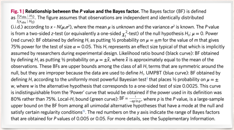
The BF redefiners provide ways to specify an “implicit alternative” the one thought to be implicitly used by statistical significance testers. The authors of (Benjamin et al. 2017) consider Bayes factors comparing a 0 point null to “classes of plausible alternatives”, where a plausible alternative is set at the value associated with high power, .75 or .8. (A few different approaches are given.) As they see it, “This H₁ represents an effect size typical of that which is implicitly assumed by researchers during experimental design”. In their view, this is the effect size that statistical significance testers assume holds if H₀ is false and H₁ true. July 26 addition: See the description in Benjamin et al. 2017 at the end of this post.

From the Bayes factor perspective, the reason for setting high power to detect δ₄, is to ensure the statistically significant result—just the point—is sufficiently probable assuming δ₄, as compared to its probability under the null H₀, set at 0.[2] They want this ratio to be around 15, 20, or 25 so that, with various priors assigned to the two hypotheses, H₁ gets a high posterior (~.95). To this end, they recommend using a p-value threshold of .005. Whether that’s a good threshold is a separate question. The problem is that a BF test is very different from a statistical significance test. Significance testers are not testing 0 vs a difference against which a test has .8 power. They are not assuming that if there is a genuine effect it is highly clinically relevant δ₄. As Senn says, this would be ludicrous. What error statistical researchers are doing is designing an experiment with a high enough probability of producing a statistically significant result D*, were the effect size as large as δ₄—one that we would be (very) unhappy to miss.

What the redefiners think they’re doing, or purport to be doing, is aligning BF tests with statistical significance tests. They aver that this allows them to argue that what’s problematic for a BF tester is also problematic for a significance tester.[3]

From the perspective of the redefiners:

“A two-sided P-value of 0.05 corresponds to Bayes factors in favor of H that range from about 2.5 to 3.4 under reasonable assumptions about H. … This is weak evidence from at least three perspectives.”

None of the three is the perspective of the statistical significance tester.

 “[W]e suspect many scientists would guess that P≈ 0.05 implies stronger support for H₁ than a Bayes factor of 2.5 to 3.4. … [With a] prior odds of 1:10, a P value of 0.05 corresponds to at least 3:1 odds (that is, the reciprocal of the product 1/10 × 3.4) in favour of the null hypothesis!”

Perhaps ‘we (Bayes factor testers) would suspect that.’ But we (statistical significance testers) would  suspect many scientists would guess that a good statistical account would not find evidence in favor of the null hypothesis of 0 when the lower bound of a .95 or .975 confidence interval exceeds 0 (and so excludes 0). We suspect they’d be very unhappy with an account that converted a method (such as statistical significance tests) that enables flagging various interesting discrepancies into a (ludicrous) test between no discrepancy and a highly clinically relevant one.[4] At the same time, the test has a low power to detect various population effects that might be of interest between 0 and δ₄.[5] As Senn reminds us, “a nonsignificant result will often mean the end of the road for a treatment. It will be lost forever. However, a treatment which shows a ‘significant’ effect will be studied further” (Senn 2007, 202).

So, listen to Senn–statistical significance testers should be careful what they wish for– but they should also be careful to question when other approaches, with very different aims, dictate what they really wish for. That would be ludicrous.

Please share your thoughts and questions in the comments.

Notes

[1] The 4 deltas (from an earlier guest post by Senn) were:

1.It is the difference we would like to observe
2. It is the difference we would like to ‘prove’ obtains
3.  It is the difference we believe obtains
4.  It is the difference you would not like to miss.

[2] Their example involves testing the mean of a normal distribution rather than testing the difference of means, but the point is analogous.

[3] See Richard Morey for a critical discussion of the statistical arguments behind redefine statistical significance.

[4] Of course there’s a big difference in what’s being inferred. The BF tester is comparing point values of the parameter; whereas the significance test is not comparative, and infers that the parameter value exceeds some value, or is less than some value. I say “of course”, but have any BF testers stopped to discuss this? I ask readers to place examples in the comments.

[5] Note too that, even if the statistically significant result just reached the .005 level, the error statistician would not infer evidence of so large a population discrepancy as large as δ₄ The p-value associated with testing that ∆ = δ₄ would be ~0.5! Ironically, from the perspective of the significance tester, the BF construal is exaggerating the evidence warranted by a just statistically significant result. Moreover, the error probability control of statistical significance tests is lost, since BFs are insensitive to gambits that alter error probabilities—at least as standardly formulated.