Monthly Archives: September 2013

Highly probable vs highly probed: Bayesian/ error statistical differences

3077175-lgA reader asks: “Can you tell me about disagreements on numbers between a severity assessment within error statistics, and a Bayesian assessment of posterior probabilities?” Sure.

There are differences between Bayesian posterior probabilities and formal error statistical measures, as well as between the latter and a severity (SEV) assessment, which differs from the standard type 1 and 2 error probabilities, p-values, and confidence levels—despite the numerical relationships. Here are some random thoughts that will hopefully be relevant for both types of differences. (Please search this blog for specifics.)

1. The most noteworthy difference is that error statistical inference makes use of outcomes other than the one observed, even after the data are available: there’s no other way to ask things like, how often would you find 1 nominally statistically significant difference in a hunting expedition over k or more factors?  Or to distinguish optional stopping with sequential trials from fixed sample size experiments.  Here’s a quote I came across just yesterday:

“[S]topping ‘when the data looks good’ can be a serious error when combined with frequentist measures of evidence. For instance, if one used the stopping rule [above]…but analyzed the data as if a fixed sample had been taken, one could guarantee arbitrarily strong frequentist ‘significance’ against H0.” (Berger and Wolpert, 1988, 77).

The worry about being guaranteed to erroneously exclude the true parameter value here is an error statistical affliction that the Bayesian is spared (even though I don’t think they can be too happy about it, especially when HPD intervals are assured of excluding the true parameter value.) See this post for an amusing note; Mayo and Kruse (2001) below; and, if interested, search the (strong)  likelihood principle, and Birnbaum.

2. Highly probable vs. highly probed. SEV doesn’t obey the probability calculus: for any test T and outcome x, the severity for both H and ~H might be horribly low. Moreover, an error statistical analysis is not in the business of probabilifying hypotheses but evaluating and controlling the capabilities of methods to discern inferential flaws (problems with linking statistical and scientific claims, problems of interpreting statistical tests and estimates, and problems of underlying model assumptions). This is the basis for applying what may be called the Severity principle. Continue reading

Categories: Bayesian/frequentist, Error Statistics, P-values, Philosophy of Statistics, Statistics, Stephen Senn, strong likelihood principle | 41 Comments

Blog Contents: August 2013

IMG_0244August 2013
(8/1) Blogging (flogging?) the SLP: Response to Reply- Xi’an Robert
(8/5) At the JSM: 2013 International Year of Statistics
(8/6) What did Nate Silver just say? Blogging the JSM
(8/9) 11th bullet, multiple choice question, and last thoughts on the JSM
(8/11) E.S. Pearson: “Ideas came into my head as I sat on a gate overlooking an experimental blackcurrant plot”
(8/13) Blogging E.S. Pearson’s Statistical Philosophy
(8/15) A. Spanos: Egon Pearson’s Neglected Contributions to Statistics
(8/17) Gandenberger: How to Do Philosophy That Matters (guest post)
(8/21) Blog contents: July, 2013
(8/22) PhilStock: Flash Freeze
(8/22) A critical look at “critical thinking”: deduction and induction
(8/28) Is being lonely unnatural for slim particles? A statistical argument
(8/31) Overheard at the comedy hour at the Bayesian retreat-2 years on

Categories: Announcement, Statistics | Leave a comment

Gelman est effectivement une erreur statistician

eiffel-tower-design-bill-cannonA reader calls my attention to Andrew Gelman’s blog announcing a talk that he’s giving today in French: “Philosophie et practique de la statistique bayésienne. He blogs:

I’ll try to update the slides a bit since a few years ago, to add some thoughts I’ve had recently about problems with noninformative priors, even in simple settings.

The location of the talk will not be convenient for most of you, but anyone who comes to the trouble of showing up will have the opportunity to laugh at my accent.

P.S. For those of you who are interested in the topic but can’t make it to the talk, I recommend these two papers on my non-inductive Bayesian philosophy:

[2013] Philosophy and the practice of Bayesian statistics (with discussion). British Journal of Mathematical and Statistical Psychology, 8–18. (Andrew Gelman and Cosma Shalizi)
[2013] Rejoinder to discussion. (Andrew Gelman and Cosma Shalizi)

[2011] Induction and deduction in Bayesian data analysis. Rationality, Markets and Morals}, special topic issue “Statistical Science and Philosophy of Science: Where Do (Should) They Meet In 2011 and Beyond?” (Andrew Gelman)

These papers, especially Gelman (2011), are discussed on this blog (in “U-Phils”). Comments by Senn, Wasserman, and Hennig may be found here, and here,with a response here (please use search for more).

As I say in my comments on Gelman and Shalizi, I think Gelman’s position is (or intends to be) inductive– in the sense of being ampliative (going beyond the data)– but simply not probabilist, i.e., not a matter of updating priors. (A blog post is here)[i]. Here’s a snippet from my comments: Continue reading

Categories: Error Statistics, Gelman | Tags: | 17 Comments

Barnard’s Birthday: background, likelihood principle, intentions

G.A. Barnard: 23 Sept.1915 – 9 Aug.2002

Reblog (year ago) : G.A. Barnard’s birthday is today, so here’s a snippet of his discussion with Savage (1962) (link below [i]) that connects to some earlier issues: stopping rules, likelihood principle, and background information here and here (at least of one type). (A few other Barnard links on this blog are below* .) Happy Birthday George!

Barnard: I have been made to think further about this issue of the stopping rule since I first suggested that the stopping rule was irrelevant (Barnard 1947a,b). This conclusion does not follow only from the subjective theory of probability; it seems to me that the stopping rule is irrelevant in certain circumstances.  Since 1947 I have had the great benefit of a long correspondence—not many letters because they were not very frequent, but it went on over a long time—with Professor Bartlett, as a result of which I am considerably clearer than I was before. My feeling is that, as I indicated [on p. 42], we meet with two sorts of situation in applying statistics to data One is where we want to have a single hypothesis with which to confront the data. Do they agree with this hypothesis or do they not? Now in that situation you cannot apply Bayes’s theorem because you have not got any alternatives to think about and specify—not yet. I do not say they are not specifiable—they are not specified yet. And in that situation it seems to me the stopping rule is relevant.

In particular, suppose somebody sets out to demonstrate the existence of extrasensory perception and says ‘I am going to go on until I get a one in ten thousand significance level’. Knowing that this is what he is setting out to do would lead you to adopt a different test criterion. What you would look at would not be the ratio of successes obtained, but how long it took him to obtain it. And you would have a very simple test of significance which said if it took you so long to achieve this increase in the score above the chance fraction, this is not at all strong evidence for E.S.P., it is very weak evidence. And the reversing of the choice of test criteria would I think overcome the difficulty.

This is the answer to the point Professor Savage makes; he says why use one method when you have vague knowledge, when you would use a quite different method when you have precise knowledge. It seem to me the answer is that you would use one method when you have precisely determined alternatives, with which you want to compare a given hypothesis, and you use another method when you do not have these alternatives.

Savage: May I digress to say publicly that I learned the stopping-rule principle from professor Barnard, in conversation in the summer of 1952. Frankly I then thought it a scandal that anyone in the profession could advance an idea so patently wrong, even as today I can scarcely believe that some people resist an idea so patently right. I am particularly surprised to hear Professor Barnard say today that the stopping rule is irrelevant in certain circumstances only, for the argument he first gave in favour of the principle seems quite unaffected by the distinctions just discussed. The argument then was this: The design of a sequential experiment is, in the last analysis, what the experimenter actually intended to do. His intention is locked up inside his head and cannot be known to those who have to judge the experiment. Never having been comfortable with that argument, I am not advancing it myself. But if Professor Barnard still accepts it, how can he conclude that the stopping-rule principle is only sometimes valid? (emphasis added) Continue reading

Categories: Background knowledge, Likelihood Principle, phil/history of stat, Philosophy of Statistics | Leave a comment

Statistical Theater of the Absurd: “Stat on a Hot Tin Roof”

metablog old fashion typewriter

Memory lane: Did you ever consider how some of the colorful exchanges among better-known names in statistical foundations could be the basis for high literary drama in the form of one-act plays (even if appreciated by only 3-7 people in the world)? (Think of the expressionist exchange between Bohr and Heisenberg in Michael Frayn’s play Copenhagen, except here there would be no attempt at all to popularize—only published quotes and closely remembered conversations would be included, with no attempt to create a “story line”.)  Somehow I didn’t think so. But rereading some of Savage’s high-flown praise of Birnbaum’s “breakthrough” argument (for the Likelihood Principle) today, I was swept into a “(statistical) theater of the absurd” mindset.

The first one came to me in autumn 2008 while I was giving a series of seminars on philosophy of statistics at the LSE. Modeled on a disappointing (to me) performance of The Woman in Black, “A Funny Thing Happened at the [1959] Savage Forum” relates Savage’s horror at George Barnard’s announcement of having rejected the Likelihood Principle!

The current piece taking shape also features George Barnard and since tomorrow (9/23) is his birthday, I’m digging it out of “rejected posts”. It recalls our first meeting in London in 1986. I’d sent him a draft of my paper “Why Pearson Rejected the Neyman-Pearson Theory of Statistics” (later adapted as chapter 11 of EGEK) to see whether I’d gotten Pearson right. He’d traveled quite a ways, from Colchester, I think. It was June and hot, and we were up on some kind of a semi-enclosed rooftop. Barnard was sitting across from me looking rather bemused.Barnard-1979-picture

The curtain opens with Barnard and Mayo on the roof, lit by a spot mid-stage. He’s drinking (hot) tea; she, a Diet Coke. The dialogue (is what I recall from the time[i]):

 Barnard: I read your paper. I think it is quite good.  Did you know that it was I who told Fisher that Neyman-Pearson statistics had turned his significance tests into little more than acceptance procedures?

Mayo:  Thank you so much for reading my paper.  I recall a reference to you in Pearson’s response to Fisher, but I didn’t know the full extent.

Barnard: I was the one who told Fisher that Neyman was largely to blame. He shouldn’t be too hard on Egon.  His statistical philosophy, you are aware, was different from Neyman’s. Continue reading

Categories: Barnard, phil/history of stat, rejected post, Statistics | Tags: , , , , | 6 Comments

How to hire a fraudster chauffeur

images-16Would you buy a used car from this man? Probably not, but he thinks you might like to hire him as your chauffeur and brilliant conversationalist. I’m not kidding: fraudster Diederik Stapel is now offering what he calls ‘mind rides’ (see ad below video). He is prepared “to listen to what you have to say or talk to you about what fascinates, surprises or angers you”. He is already giving pedagogical talks on a train. This from Retraction Watch:

Diederik Stapel, the social psychologist who has now retracted 54 papers, recently spoke as part of the TEDx Braintrain, which took place on a trip from Maastricht to Amsterdam. Among other things, he says he lost his moral compass, but that it’s back.

Here’s a  rough translation of the chauffeur ad from Stapel’s website (source is this blog):

Always on the move, from A to B, hurried, no time for reflection, for distance, for perspective. […] Diederik offers himself as your driver and conversation partner who won’t just get you from A to B, but who would also like to add meaning and disruption to your travel time. He will […] listen to what you have to say or talk to you about what fascinates, surprises or angers you. [Slightly paraphrased for brevity—Branko]

I don’t think I’d pay to have a Stapel “disruption” added to my travel time, would you? He sounds so much as he does in “Ontsporing”[i],

[i]The following is from a review of his Ontsporing [“derailed”].

“Ontsporing provides the first glimpses of how, why, and where Stapel began. It details the first small steps that led to Stapel’s deception and highlights the fine line between research fact and fraud:

‘I was alone in my fancy office at University of Groningen.… I opened the file that contained research data I had entered and changed an unexpected 2 into a 4.… I looked at the door. It was closed.… I looked at the matrix with data and clicked my mouse to execute the relevant statistical analyses. When I saw the new results, the world had returned to being logical’. (p. 145) Continue reading

Categories: Statistical fraudbusting | 12 Comments

PhilStock: Bad news is good news on Wall St.

stock picture smaillSee rejected posts.

Categories: PhilStock, Rejected Posts | Leave a comment

“When Bayesian Inference Shatters” Owhadi and Scovel (guest post)

images-9I’m extremely grateful to Drs. Owhadi and Scovel for replying to my request for “a plain Jane” explication of their interesting paper, “When Bayesian Inference Shatters”, and especially for permission to post it. If readers want to ponder the paper awhile and send me comments for guest posts or “U-PHILS*” (by OCT 15), let me know. Feel free to comment as usual in the mean time.

—————————————-

owhadiHouman Owhadi
Professor of Applied and Computational Mathematics and Control and Dynamical Systems, Computing + Mathematical Sciences,
California Institute of Technology, USA

Clint ScovelClintpic
Senior Scientist,
Computing + Mathematical Sciences,
California Institute of Technology, USA

“When Bayesian Inference Shatters: A plain Jane explanation”

This is an attempt at a “plain Jane” presentation of the results discussed in the recent arxiv paper “When Bayesian Inference Shatters” located at http://arxiv.org/abs/1308.6306 with the following abstract:

“With the advent of high-performance computing, Bayesian methods are increasingly popular tools for the quantification of uncertainty throughout science and industry. Since these methods impact the making of sometimes critical decisions in increasingly complicated contexts, the sensitivity of their posterior conclusions with respect to the underlying models and prior beliefs is becoming a pressing question. We report new results suggesting that, although Bayesian methods are robust when the number of possible outcomes is finite or when only a finite number of marginals of the data-generating distribution are unknown, they are generically brittle when applied to continuous systems with finite information on the data-generating distribution. This brittleness persists beyond the discretization of continuous systems and suggests that Bayesian inference is generically ill-posed in the sense of Hadamard when applied to such systems: if closeness is defined in terms of the total variation metric or the matching of a finite system of moments, then (1) two practitioners who use arbitrarily close models and observe the same (possibly arbitrarily large amount of) data may reach diametrically opposite conclusions; and (2) any given prior and model can be slightly perturbed to achieve any desired posterior conclusions.”

Now, it is already known from classical Robust Bayesian Inference that Bayesian Inference has some robustness if the random outcomes live in a finite space or if the class of priors considered is finite-dimensional (i.e. what you know is infinite and what you do not know is finite). What we have shown is that if the random outcomes live in an approximation of a continuous space (for instance, when they are decimal numbers given to finite precision) and your class of priors is finite co-dimensional (i.e. what you know is finite and what you do not know may be infinite) then, if the data is observed at a fine enough resolution, the range of posterior values is the deterministic range of the quantity of interest, irrespective of the size of the data. Continue reading

Categories: Bayesian/frequentist, Statistics | 40 Comments

(Part 3) Peircean Induction and the Error-Correcting Thesis

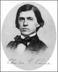
C. S. Peirce: 10 Sept, 1839-19 April, 1914

C. S. Peirce: 10 Sept, 1839-19 April, 1914

Last third of “Peircean Induction and the Error-Correcting Thesis”

Deborah G. Mayo
Transactions of the Charles S. Peirce Society 41(2) 2005: 299-319

Part 2 is here.

8. Random sampling and the uniformity of nature

We are now at the point to address the final move in warranting Peirce’s SCT. The severity or trustworthiness assessment, on which the error correcting capacity depends, requires an appropriate link (qualitative or quantitative) between the data and the data generating phenomenon, e.g., a reliable calibration of a scale in a qualitative case, or a probabilistic connection between the data and the population in a quantitative case. Establishing such a link, however, is regarded as assuming observed regularities will persist, or making some “uniformity of nature” assumption—the bugbear of attempts to justify induction.

But Peirce contrasts his position with those favored by followers of Mill, and “almost all logicians” of his day, who “commonly teach that the inductive conclusion approximates to the truth because of the uniformity of nature” (2.775). Inductive inference, as Peirce conceives it (i.e., severe testing) does not use the uniformity of nature as a premise. Rather, the justification is sought in the manner of obtaining data. Justifying induction is a matter of showing that there exist methods with good error probabilities. For this it suffices that randomness be met only approximately, that inductive methods check their own assumptions, and that they can often detect and correct departures from randomness.

… It has been objected that the sampling cannot be random in this sense. But this is an idea which flies far away from the plain facts. Thirty throws of a die constitute an approximately random sample of all the throws of that die; and that the randomness should be approximate is all that is required. (1.94)

Peirce backs up his defense with robustness arguments. For example, in an (attempted) Binomial induction, Peirce asks, “what will be the effect upon inductive inference of an imperfection in the strictly random character of the sampling” (2.728). What if, for example, a certain proportion of the population had twice the probability of being selected? He shows that “an imperfection of that kind in the random character of the sampling will only weaken the inductive conclusion, and render the concluded ratio less determinate, but will not necessarily destroy the force of the argument completely” (2.728). This is particularly so if the sample mean is near 0 or 1. In other words, violating experimental assumptions may be shown to weaken the trustworthiness or severity of the proceeding, but this may only mean we learn a little less.

Yet a further safeguard is at hand:

Nor must we lose sight of the constant tendency of the inductive process to correct itself. This is of its essence. This is the marvel of it. …even though doubts may be entertained whether one selection of instances is a random one, yet a different selection, made by a different method, will be likely to vary from the normal in a different way, and if the ratios derived from such different selections are nearly equal, they may be presumed to be near the truth. (2.729)

Here, the marvel is an inductive method’s ability to correct the attempt at random sampling. Still, Peirce cautions, we should not depend so much on the self-correcting virtue that we relax our efforts to get a random and independent sample. But if our effort is not successful, and neither is our method robust, we will probably discover it. “This consideration makes it extremely advantageous in all ampliative reasoning to fortify one method of investigation by another” (ibid.).

“The Supernal Powers Withhold Their Hands And Let Me Alone”

Peirce turns the tables on those skeptical about satisfying random sampling—or, more generally, satisfying the assumptions of a statistical model. He declares himself “willing to concede, in order to concede as much as possible, that when a man draws instances at random, all that he knows is that he tried to follow a certain precept” (2.749). There might be a “mysterious and malign connection between the mind and the universe” that deliberately thwarts such efforts. He considers betting on the game of rouge et noire: “could some devil look at each card before it was turned, and then influence me mentally” to bet or not, the ratio of successful bets might differ greatly from 0.5. But, as Peirce is quick to point out, this would equally vitiate deductive inferences about the expected ratio of successful bets.

Consider our informal example of weighing with calibrated scales. If I check the properties of the scales against known, standard weights, then I can check if my scales are working in a particular case. Were the scales infected by systematic error, I would discover this by finding systematic mismatches with the known weights; I could then subtract it out in measurements. That scales have given properties where I know the object’s weight indicates they have the same properties when the weights are unknown, lest I be forced to assume that my knowledge or ignorance somehow influences the properties of the scale. More generally, Peirce’s insightful argument goes, the experimental procedure thus confirmed where the measured property is known must work as well when it is unknown unless a mysterious and malign demon deliberately thwarts my efforts. Continue reading

Categories: C.S. Peirce, Error Statistics, phil/history of stat | 6 Comments

(Part 2) Peircean Induction and the Error-Correcting Thesis

C. S. Peirce 9/10/1839 – 4/19/1914

C. S. Peirce
9/10/1839 – 4/19/1914

Continuation of “Peircean Induction and the Error-Correcting Thesis”

Deborah G. Mayo
Transactions of the Charles S. Peirce Society: A Quarterly Journal in American Philosophy, Volume 41, Number 2, 2005, pp. 299-319

Part 1 is here.

There are two other points of confusion in critical discussions of the SCT, that we may note here:

I. The SCT and the Requirements of Randomization and Predesignation

The concern with “the trustworthiness of the proceeding” for Peirce like the concern with error probabilities (e.g., significance levels) for error statisticians generally, is directly tied to their view that inductive method should closely link inferences to the methods of data collection as well as to how the hypothesis came to be formulated or chosen for testing.

This account of the rationale of induction is distinguished from others in that it has as its consequences two rules of inductive inference which are very frequently violated (1.95) namely, that the sample be (approximately) random and that the property being tested not be determined by the particular sample x— i.e., predesignation.

The picture of Peircean induction that one finds in critics of the SCT disregards these crucial requirements for induction: Neither enumerative induction nor H-D testing, as ordinarily conceived, requires such rules. Statistical significance testing, however, clearly does.

Suppose, for example that researchers wishing to demonstrate the benefits of HRT search the data for factors on which treated women fare much better than untreated, and finding one such factor they proceed to test the null hypothesis:

H0: there is no improvement in factor F (e.g. memory) among women treated with HRT.

Having selected this factor for testing solely because it is a factor on which treated women show impressive improvement, it is not surprising that this null hypothesis is rejected and the results taken to show a genuine improvement in the population. However, when the null hypothesis is tested on the same data that led it to be chosen for testing, it is well known, a spurious impression of a genuine effect easily results. Suppose, for example, that 20 factors are examined for impressive-looking improvements among HRT-treated women, and the one difference that appears large enough to test turns out to be significant at the 0.05 level. The actual significance level—the actual probability of reporting a statistically significant effect when in fact the null hypothesis is true—is not 5% but approximately 64% (Mayo 1996, Mayo and Kruse 2001, Mayo and Cox 2006). To infer the denial of H0, and infer there is evidence that HRT improves memory, is to make an inference with low severity (approximately 0.36).

II Understanding the “long-run error correcting” metaphor

Discussions of Peircean ‘self-correction’ often confuse two interpretations of the ‘long-run’ error correcting metaphor, even in the case of quantitative induction: (a) Asymptotic self-correction (as n approaches ∞): In this construal, it is imagined that one has a sample, say of size n=10, and it is supposed that the SCT assures us that as the sample size increases toward infinity, one gets better and better estimates of some feature of the population, say the mean. Although this may be true, provided assumptions of a statistical model (e.g., the Binomial) are met, it is not the sense intended in significance-test reasoning nor, I maintain, in Peirce’s SCT. Peirce’s idea, instead, gives needed insight for understanding the relevance of ‘long-run’ error probabilities of significance tests to assess the reliability of an inductive inference from a specific set of data, (b) Error probabilities of a test: In this construal, one has a sample of size n, say 10, and imagines hypothetical replications of the experiment—each with samples of 10. Each sample of 10 gives a single value of the test statistic d(X), but one can consider the distribution of values that would occur in hypothetical repetitions (of the given type of sampling). The probability distribution of d(X) is called the sampling distribution, and the correct calculation of the significance level is an example of how tests appeal to this distribution: Thanks to the relationship between the observed d(x) and the sampling distribution of d(X), the former can be used to reliably probe the correctness of statistical hypotheses (about the procedure) that generated the particular 10-fold sample. That is what the SCT is asserting.

It may help to consider a very informal example. Suppose that weight gain is measured by 10 well-calibrated and stable methods, possibly using several measuring instruments and the results show negligible change over a test period of interest. This may be regarded as grounds for inferring that the individual’s weight gain is negligible within limits set by the sensitivity of the scales. Why? While it is true that by averaging more and more weight measurements, i.e., an eleventh, twelfth, etc., one would get asymptotically close to the true weight, that is not the rationale for the particular inference. The rationale is rather that the error probabilistic properties of the weighing procedure (the probability of ten-fold weighings erroneously failing to show weight change) inform one of the correct weight in the case at hand, e.g., that a 0 observed weight increase passes the “no-weight gain” hypothesis with high severity. Continue reading

Categories: Bayesian/frequentist, C.S. Peirce, Error Statistics, Statistics | 5 Comments

Peircean Induction and the Error-Correcting Thesis (Part I)

C. S. Peirce: 10 Sept, 1839-19 April, 1914

C. S. Peirce: 10 Sept, 1839-19 April, 1914

Today is C.S. Peirce’s birthday. I hadn’t blogged him before, but he’s one of my all time heroes. You should read him: he’s a treasure chest on essentially any topic. I’ll blog the main sections of a (2005) paper over the next few days. It’s written for a very general philosophical audience; the statistical parts are pretty informal. Happy birthday Peirce.

Peircean Induction and the Error-Correcting Thesis
Deborah G. Mayo
Transactions of the Charles S. Peirce Society: A Quarterly Journal in American Philosophy, Volume 41, Number 2, 2005, pp. 299-319

Peirce’s philosophy of inductive inference in science is based on the idea that what permits us to make progress in science, what allows our knowledge to grow, is the fact that science uses methods that are self-correcting or error-correcting:

Induction is the experimental testing of a theory. The justification of it is that, although the conclusion at any stage of the investigation may be more or less erroneous, yet the further application of the same method must correct the error. (5.145)

Inductive methods—understood as methods of experimental testing—are justified to the extent that they are error-correcting methods. We may call this Peirce’s error-correcting or self-correcting thesis (SCT):

Self-Correcting Thesis SCT: methods for inductive inference in science are error correcting; the justification for inductive methods of experimental testing in science is that they are self-correcting.

Peirce’s SCT has been a source of fascination and frustration. By and large, critics and followers alike have denied that Peirce can sustain his SCT as a way to justify scientific induction: “No part of Peirce’s philosophy of science has been more severely criticized, even by his most sympathetic commentators, than this attempted validation of inductive methodology on the basis of its purported self-correctiveness” (Rescher 1978, p. 20).

In this paper I shall revisit the Peircean SCT: properly interpreted, I will argue, Peirce’s SCT not only serves its intended purpose, it also provides the basis for justifying (frequentist) statistical methods in science. While on the one hand, contemporary statistical methods increase the mathematical rigor and generality of Peirce’s SCT, on the other, Peirce provides something current statistical methodology lacks: an account of inductive inference and a philosophy of experiment that links the justification for statistical tests to a more general rationale for scientific induction. Combining the mathematical contributions of modern statistics with the inductive philosophy of Peirce, sets the stage for developing an adequate justification for contemporary inductive statistical methodology.

2. Probabilities are assigned to procedures not hypotheses

Peirce’s philosophy of experimental testing shares a number of key features with the contemporary (Neyman and Pearson) Statistical Theory: statistical methods provide, not means for assigning degrees of probability, evidential support, or confirmation to hypotheses, but procedures for testing (and estimation), whose rationale is their predesignated high frequencies of leading to correct results in some hypothetical long-run. A Neyman and Pearson (NP) statistical test, for example, instructs us “To decide whether a hypothesis, H, of a given type be rejected or not, calculate a specified character, x0, of the observed facts; if x> x0 reject H; if x< x0 accept H.” Although the outputs of N-P tests do not assign hypotheses degrees of probability, “it may often be proved that if we behave according to such a rule … we shall reject H when it is true not more, say, than once in a hundred times, and in addition we may have evidence that we shall reject H sufficiently often when it is false” (Neyman and Pearson, 1933, p.142).[i]

The relative frequencies of erroneous rejections and erroneous acceptances in an actual or hypothetical long run sequence of applications of tests are error probabilities; we may call the statistical tools based on error probabilities, error statistical tools. In describing his theory of inference, Peirce could be describing that of the error-statistician:

The theory here proposed does not assign any probability to the inductive or hypothetic conclusion, in the sense of undertaking to say how frequently that conclusion would be found true. It does not propose to look through all the possible universes, and say in what proportion of them a certain uniformity occurs; such a proceeding, were it possible, would be quite idle. The theory here presented only says how frequently, in this universe, the special form of induction or hypothesis would lead us right. The probability given by this theory is in every way different—in meaning, numerical value, and form—from that of those who would apply to ampliative inference the doctrine of inverse chances. (2.748)

The doctrine of “inverse chances” alludes to assigning (posterior) probabilities in hypotheses by applying the definition of conditional probability (Bayes’s theorem)—a computation requires starting out with a (prior or “antecedent”) probability assignment to an exhaustive set of hypotheses:

If these antecedent probabilities were solid statistical facts, like those upon which the insurance business rests, the ordinary precepts and practice [of inverse probability] would be sound. But they are not and cannot be statistical facts. What is the antecedent probability that matter should be composed of atoms? Can we take statistics of a multitude of different universes? (2.777)

For Peircean induction, as in the N-P testing model, the conclusion or inference concerns a hypothesis that either is or is not true in this one universe; thus, assigning a frequentist probability to a particular conclusion, other than the trivial ones of 1 or 0, for Peirce, makes sense only “if universes were as plentiful as blackberries” (2.684). Thus the Bayesian inverse probability calculation seems forced to rely on subjective probabilities for computing inverse inferences, but “subjective probabilities” Peirce charges “express nothing but the conformity of a new suggestion to our prepossessions, and these are the source of most of the errors into which man falls, and of all the worse of them” (2.777).

Hearing Pierce contrast his view of induction with the more popular Bayesian account of his day (the Conceptualists), one could be listening to an error statistician arguing against the contemporary Bayesian (subjective or other)—with one important difference. Today’s error statistician seems to grant too readily that the only justification for N-P test rules is their ability to ensure we will rarely take erroneous actions with respect to hypotheses in the long run of applications. This so called inductive behavior rationale seems to supply no adequate answer to the question of what is learned in any particular application about the process underlying the data. Peirce, by contrast, was very clear that what is really wanted in inductive inference in science is the ability to control error probabilities of test procedures, i.e., “the trustworthiness of the proceeding”. Moreover it is only by a faulty analogy with deductive inference, Peirce explains, that many suppose that inductive (synthetic) inference should supply a probability to the conclusion: “… in the case of analytic inference we know the probability of our conclusion (if the premises are true), but in the case of synthetic inferences we only know the degree of trustworthiness of our proceeding (“The Probability of Induction” 2.693).

Knowing the “trustworthiness of our inductive proceeding”, I will argue, enables determining the test’s probative capacity, how reliably it detects errors, and the severity of the test a hypothesis withstands. Deliberately making use of known flaws and fallacies in reasoning with limited and uncertain data, tests may be constructed that are highly trustworthy probes in detecting and discriminating errors in particular cases. This, in turn, enables inferring which inferences about the process giving rise to the data are and are not warranted: an inductive inference to hypothesis H is warranted to the extent that with high probability the test would have detected a specific flaw or departure from what H asserts, and yet it did not.

3. So why is justifying Peirce’s SCT thought to be so problematic?

You can read Section 3 here. (it’s not necessary for understanding the rest).

4. Peircean induction as severe testing

… [I]nduction, for Peirce, is a matter of subjecting hypotheses to “the test of experiment” (7.182).

The process of testing it will consist, not in examining the facts, in order to see how well they accord with the hypothesis, but on the contrary in examining such of the probable consequences of the hypothesis … which would be very unlikely or surprising in case the hypothesis were not true. (7.231)

When, however, we find that prediction after prediction, notwithstanding a preference for putting the most unlikely ones to the test, is verified by experiment,…we begin to accord to the hypothesis a standing among scientific results.

This sort of inference it is, from experiments testing predictions based on a hypothesis, that is alone properly entitled to be called induction. (7.206)

While these and other passages are redolent of Popper, Peirce differs from Popper in crucial ways. Peirce, unlike Popper, is primarily interested not in falsifying claims but in the positive pieces of information provided by tests, with “the corrections called for by the experiment” and with the hypotheses, modified or not, that manage to pass severe tests. For Popper, even if a hypothesis is highly corroborated (by his lights), he regards this as at most a report of the hypothesis’ past performance and denies it affords positive evidence for its correctness or reliability. Further, Popper denies that he could vouch for the reliability of the method he recommends as “most rational”—conjecture and refutation. Indeed, Popper’s requirements for a highly corroborated hypothesis are not sufficient for ensuring severity in Peirce’s sense (Mayo 1996, 2003, 2005). Where Popper recoils from even speaking of warranted inductions, Peirce conceives of a proper inductive inference as what had passed a severe test—one which would, with high probability, have detected an error if present.

In Peirce’s inductive philosophy, we have evidence for inductively inferring a claim or hypothesis H when not only does H “accord with” the data x; but also, so good an accordance would very probably not have resulted, were H not true. In other words, we may inductively infer H when it has withstood a test of experiment that it would not have withstood, or withstood so well, were H not true (or were a specific flaw present). This can be encapsulated in the following severity requirement for an experimental test procedure, ET, and data set x.

Hypothesis H passes a severe test with x iff (firstly) x accords with H and (secondly) the experimental test procedure ET would, with very high probability, have signaled the presence of an error were there a discordancy between what H asserts and what is correct (i.e., were H false).

The test would “have signaled an error” by having produced results less accordant with H than what the test yielded. Thus, we may inductively infer H when (and only when) H has withstood a test with high error detecting capacity, the higher this probative capacity, the more severely H has passed. What is assessed (quantitatively or qualitatively) is not the amount of support for H but the probative capacity of the test of experiment ET (with regard to those errors that an inference to H is declaring to be absent)……….

You can read the rest of Section 4 here.

5. The path from qualitative to quantitative induction

In my understanding of Peircean induction, the difference between qualitative and quantitative induction is really a matter of degree, according to whether their trustworthiness or severity is quantitatively or only qualitatively ascertainable. This reading not only neatly organizes Peirce’s typologies of the various types of induction, it underwrites the manner in which, within a given classification, Peirce further subdivides inductions by their “strength”.

(I) First-Order, Rudimentary or Crude Induction

Consider Peirce’s First Order of induction: the lowest, most rudimentary form that he dubs, the “pooh-pooh argument”. It is essentially an argument from ignorance: Lacking evidence for the falsity of some hypothesis or claim H, provisionally adopt H. In this very weakest sort of induction, crude induction, the most that can be said is that a hypothesis would eventually be falsified if false. (It may correct itself—but with a bang!) It “is as weak an inference as any that I would not positively condemn” (8.237). While uneliminable in ordinary life, Peirce denies that rudimentary induction is to be included as scientific induction. Without some reason to think evidence of H‘s falsity would probably have been detected, were H false, finding no evidence against H is poor inductive evidence for H. H has passed only a highly unreliable error probe. Continue reading

Categories: Bayesian/frequentist, C.S. Peirce, Error Statistics, Statistics | 6 Comments

First blog: “Did you hear the one about the frequentist…”? and “Frequentists in Exile”

metablog old fashion typewriterDear Reader: Tonight marks the 2-year anniversary of this blog; so I’m reblogging my very first posts from 9/3/11 here and here (from the rickety old blog site)*. (One was the “about”.) The current blog was included once again in the top 50 statistics blogs. Amazingly, I have received e-mails from different parts of the world describing experimental recipes for the special concoction we exiles favor!  (Mine is here.) If you can fly over to the Elbar Room, please join us: I’m treating everyone to doubles of Elbar Grease!  Thanks for reading and contributing! D. G. Mayo

(*The old blogspot is a big mix; it was before Rejected blogs. Yes, I still use this old typewriter [ii])

“Overheard at the Comedy Club at the Bayesian Retreat” 9/3/11 by D. Mayoimages-3

“Did you hear the one about the frequentist . . .

  • “who claimed that observing “heads” on a biased coin that lands heads with probability .05 is evidence of a statistically significant improvement over the standard treatment of diabetes, on the grounds that such an event occurs with low probability (.05)?”

or

  • “who defended the reliability of his radiation reading, despite using a broken radiometer, on the grounds that most of the time he uses one that works, so on average he’s pretty reliable?”

Such jests may work for an after-dinner laugh, but if it turns out that, despite being retreads of “straw-men” fallacies, they form the basis of why some reject frequentist methods, then they are not such a laughing matter.   But surely the drubbing of frequentist methods could not be based on a collection of howlers, could it?  I invite the curious reader to stay and find out.

If we are to take the criticisms seriously, and put to one side the possibility that they are deliberate distortions of frequentist statistical methods, we need to identify their sources. To this end I consider two interrelated areas around which to organize foundational issues in statistics: (1) the roles of probability in induction and inference, and (2) the nature and goals of statistical inference in science or learning. Frequentist sampling statistics, which I prefer to call “error statistics,” continues to be raked over the coals in the foundational literature, but with little scrutiny of the presuppositions about goals and methods, without which the criticisms lose all force.

First, there is the supposition that an adequate account must assign degrees of probability to hypotheses, an assumption often called probabilism. Second, there is the assumption that the main, if not the only, goal of error-statistical methods is to evaluate long-run error rates.   Given the wide latitude with which some critics define “controlling long-run error,” it is not surprising to find them arguing that (i) error statisticians approve of silly methods, and/or (ii) rival (e.g., Bayesian) accounts also satisfy error statistical demands. Absent this sleight of hand, Bayesian celebrants would have to go straight to the finale of their entertainment hour: a rousing rendition of “There’s No Theorem Like Bayes’s Theorem.”

Never mind that frequentists have responded to these criticisms, they keep popping up (verbatim) in many Bayesian textbooks and articles on philosophical foundations. The difficulty of articulating a statistical philosophy that fully explains the basis for both (i)  insisting on error-statistical guarantees, while (ii) avoiding pathological examples in practice, has turned many a frequentist away from venturing into foundational battlegrounds.  Some even concede the distorted perspectives drawn from overly literal and radical expositions of what Fisher, Neyman, and Pearson “really thought”.  Many others just find the “statistical wars” distasteful.

Here is where I view my contribution—as a philosopher of science—to the long-standing debate: not merely to call attention to the howlers that pass as legitimate criticisms of frequentist error statistics, but also to sketch the main lines of an alternative statistical philosophy within which to better articulate the roles and value of frequentist tools. Let me be clear that I do not consider this the only philosophical framework for frequentist statistics—different terminology could do as well.  I will consider myself successful if I can provide one way of building, or one standpoint from which to build, a frequentist, error- statistical philosophy.

But given this is a blog, I shall be direct and to the point: I hope to cultivate the interests of others who might want to promote intellectual honesty within a generally very lopsided philosophical debate.  I will begin with the first entry to the comedy routine, as it is put forth by leading Bayesians……

___________________________________________

“Frequentists in Exile” 9/3/11 by D. Mayo

Confronted with the position that “arguments for this personalistic theory were so persuasive that anything to any extent inconsistent with that theory should be discarded” (Cox 2006, 196), frequentists might have seen themselves in a kind of exile when it came to foundations, even those who had been active in the dialogues of an earlier period [i].  Sometime around the late 1990s there were signs that this was changing.  Regardless of the explanation, the fact that it did occur and is occurring is of central importance to statistical philosophy.

Now that Bayesians have stepped off their a priori pedestal, it may be hoped that a genuinely deep scrutiny of the frequentist and Bayesian accounts will occur.  In some corners of practice it appears that frequentist error statistical foundations are being discovered anew.  Perhaps frequentist foundations, never made fully explicit, but at most lying deep below the ocean floor, are finally being disinterred.  But let’s learn from some of the mistakes in the earlier attempts to understand it.  With this goal I invite you to join me in some deep water drilling, here as I cast about on my Isle of Elba.

Cox, D. R. (2006), Principles of Statistical Inference, CUP.

________________________________________________

[i] Yes, that’s the Elba connection: Napolean’s exile (from which he returned to fight more battles).

[ii] I have discovered a very reliable antique typewriter shop in Oxford that was able to replace the two missing typewriter keys. So long as my “ribbons” and carbon sheets don’t run out, I’m set.

Categories: Comedy, Error Statistics | Tags: , , , | 40 Comments

Stephen Senn: Open Season (guest post)

Stephen SennStephen Senn
Head, Methodology and Statistics Group,
Competence Center for Methodology and Statistics (CCMS),
Luxembourg

“Open Season”

The recent joint statement(1) by the Pharmaceutical Research and Manufacturers of America (PhRMA) and the European Federation of Pharmaceutical Industries and Associations(EFPIA) represents a further step in what has been a slow journey towards (one assumes) will be the achieved  goal of sharing clinical trial data. In my inaugural lecture of 1997 at University College London I called for all pharmaceutical companies to develop a policy for sharing trial results and I have repeated this in many places since(2-5). Thus I can hardly complain if what I have been calling for for over 15 years is now close to being achieved.

However, I have now recently been thinking about it again and it seems to me that there are some problems that need to be addressed. One is the issue of patient confidentiality. Ideally, covariate information should be exploitable as such often increases the precision of inferences and also the utility of decisions based upon them since they (potentially) increase the possibility of personalising medical interventions. However, providing patient-level data increases the risk of breaching confidentiality. This is a complicated and difficult issue about which, however, I have nothing useful to say. Instead I want to consider another matter. What will be the influence on the quality of the inferences we make of enabling many subsequent researchers to analyse the same data?

One of the reasons that many researchers have called for all trials to be published is that trials that are missing tend to be different from those that are present. Thus there is a bias in summarising evidence from published trial only and it can be a difficult task with no guarantee of success to identify those that have not been published. This is a wider reflection of the problem of missing data within trials. Such data have long worried trialists and the Food and Drug Administration (FDA) itself has commissioned a report on the subject from leading experts(6). On the European side the Committee for Medicinal Products for Human Use (CHMP) has a guideline dealing with it(7).

However, the problem is really a particular example of data filtering and it also applies to statistical analysis. If the analyses that are present have been selected from a wider set, then there is a danger that they do not provide an honest reflection of the message that is in the data. This problem is known as that of multiplicity and there is a huge literature dealing with it, including regulatory guidance documents(8, 9).

Within drug regulation this is dealt with by having pre-specified analyses. The broad outlines of these are usually established in the trial protocol and the approach is then specified in some detail in the statistical analysis plan which is required to be finalised before un-blinding of the data. The strategies used to control for multiplicity will involve some combination of defining a significance testing route (an order in which test must be performed and associated decision rules) and reduction of the required level of significance to detect an event.

I am not a great fan of these manoeuvres, which can be extremely complex. One of my objections is that it is effectively assumed that the researchers who chose them are mandated to circumscribe the inferences that scientific posterity can make(10). I take the rather more liberal view that provided that everything that is tested is reported one can test as much as one likes. The problem comes if there is selective use of results and in particular selective reporting. Nevertheless, I would be the first to concede the value of pre-specification in clarifying the thinking of those about to embark on conducting a clinical trial and also in providing a ‘template of trust’ for the regulator when provided with analyses by the sponsor.

However, what should be our attitude to secondary analyses? From one point of view these should be welcome. There is always value in looking at data from different perspectives and indeed this can be one way of strengthening inferences in the way suggested nearly 50 years ago by Platt(11). There are two problems, however. First, not all perspectives are equally valuable. Some analyses in the future, no doubt, will be carried out by those with little expertise and in some cases, perhaps, by those with a particular viewpoint to justify. There is also the danger that some will carry out multiple analyses (of which, when one consider the possibility of changing endpoints, performing transformations, choosing covariates and modelling framework there are usually a great number) but then only present those that are ‘interesting’. It is precisely to avoid this danger that the ritual of pre-specified analysis is insisted upon by regulators. Must we also insist upon it for those seeking to reanalyse?

To do so would require such persons to do two things. First, they would have to register the analysis plan before being granted access to the data. Second, they would have to promise to make the analysis results available, otherwise we will have a problem of missing analyses to go with the problem of missing trials. I think that it is true to say that we are just beginning to feel our way with this. It may be that the chance has been lost and that the whole of clinical research will be ‘world wide webbed’: there will be a mass of information out there but we just don’t know what to believe. Whatever happens the era of privileged statistical analyses by the original data collectors is disappearing fast.

[Ed. note: Links to some earlier related posts by Prof. Senn are:  “Casting Stones” 3/7/13, “Also Smith & Jones” 2/23/13, and “Fooling the Patient: An Unethical Use of Placebo?” 8/2/12 .]

References

1. PhRMA, EFPIA. Principles for Responsible Clinical Trial Data Sharing. PhRMA; 2013 [cited 2013 31 August]; Available from: http://phrma.org/sites/default/files/pdf/PhRMAPrinciplesForResponsibleClinicalTrialDataSharing.pdf.

2. Senn SJ. Statistical quality in analysing clinical trials. Good Clinical Practice Journal. [Research Paper]. 2000;7(6):22-6.

3. Senn SJ. Authorship of drug industry trials. Pharm Stat. [Editorial]. 2002;1:5-7.

4. Senn SJ. Sharp tongues and bitter pills. Significance. [Review]. 2006 September 2006;3(3):123-5.

5. Senn SJ. Pharmaphobia: fear and loathing of pharmaceutical research. [pdf] 1997 [updated 31 August 2013; cited 2013 31 August ]; Updated version of paper originally published on PharmInfoNet].

6. Little RJ, D’Agostino R, Cohen ML, Dickersin K, Emerson SS, Farrar JT, et al. The prevention and treatment of missing data in clinical trials. N Engl J Med. 2012 Oct 4;367(14):1355-60.

7. Committee for Medicinal Products for Human Use (CHMP). Guideline on Missing Data in Confirmatory Clinical Trials London: European Medicine Agency; 2010. p. 1-12.

8. Committee for Proprietary Medicinal Products. Points to consider on multiplicity issues in clinical trials. London: European Medicines Evaluation Agency2002.

9. International Conference on Harmonisation. Statistical principles for clinical trials (ICH E9). Statistics in Medicine. 1999;18:1905-42.

10. Senn S, Bretz F. Power and sample size when multiple endpoints are considered. Pharm Stat. 2007 Jul-Sep;6(3):161-70.

11. Platt JR. Strong Inference: Certain systematic methods of scientific thinking may produce much more rapid progress than others. Science. 1964 Oct 16;146(3642):347-53.

Categories: evidence-based policy, science communication, Statistics, Stephen Senn | 6 Comments

Gelman’s response to my comment on Jaynes

3-d red yellow puzzle people (E&I)Gelman responds to the comment[i] I made on my 8/31/13 post:
Popper and Jaynes
Posted by Andrew on 3 September 2013
Deborah Mayo quotes me as saying, “Popper has argued (convincingly, in my opinion) that scientific inference is not inductive but deductive.” She then follows up with:

Gelman employs significance test-type reasoning to reject a model when the data sufficiently disagree.

Now, strictly speaking, a model falsification, even to inferring something as weak as “the model breaks down,” is not purely deductive, but Gelman is right to see it as about as close as one can get, in statistics, to a deductive falsification of a model. But where does that leave him as a Jaynesian?

My reply:

I was influenced by reading a toy example from Jaynes’s book where he sets up a model (for the probability of a die landing on each of its six sides) based on first principles, then presents some data that contradict the model, then expands the model.

I’d seen very little of this sort of this reasoning before in statistics! In physics it’s the standard way to go: you set up a model based on physical principles and some simplifications (for example, in a finite-element model you assume the various coefficients aren’t changing over time, and you assume stability within each element), then if the model doesn’t quite work, you figure out what went wrong and you make it more realistic.

But in statistics we weren’t usually seeing this. Instead, model checking typically was placed in the category of “hypothesis testing,” where the rejection was the goal. Models to be tested were straw man, build up only to be rejected. You can see this, for example, in social science papers that list research hypotheses that are not the same as the statistical “hypotheses” being tested. A typical research hypothesis is “Y causes Z,” with the corresponding statistical hypothesis being “Y has no association with Z after controlling for X.” Jaynes’s approach—or, at least, what I took away from Jaynes’s presentation—was more simpatico to my way of doing science. And I put a lot of effort into formalizing this idea, so that the kind of modeling I talk and write about can be the kind of modeling I actually do.

I don’t want to overstate this—as I wrote earlier, Jaynes is no guru—but I do think this combination of model building and checking is important. Indeed, just as a chicken is said to be an egg’s way of making another egg, we can view inference as a way of sharpening the implications of an assumed model so that it can better be checked.

P.S. In response to Larry’s post here, let me give a quick +1 to this comment and also refer to this post, which remains relevant 3 years later.

I still don’t see how one learns about falsification from Jaynes when he alleges that the entailment of x from H disappears once H is rejected. But put that aside. In my quote from Gelman 2011, he was alluding to simple significance tests–without an alternative–for checking consistency of a model; whereas, he’s now saying what he wants is to infer an alternative model, and furthermore suggests one doesn’t see this in statistical hypotheses tests. But of course Neyman-Pearson testing always has an alternative, and even Fisherian simple significance tests generally indicate a direction of departure. However, neither type of statistical test method would automatically license going directly from a rejection of one statistical hypotheses to inferring an alternative model that was constructed to account for the misfit. A parametric discrepancy,δ, from a null may be indicated if the test very probably would not have resulted in so large an observed difference, were such a discrepancy absent (i.e., when the inferred alternative passes severely). But I’m not sure Gelman is limiting himself to such alternatives.

As I wrote in a follow-up comment: “there’s no warrant to infer a particular model that happens to do a better job fitting the data x–at least on x alone. Insofar as there are many alternatives that could patch things up, an inference to one particular alternative fails to pass with severity. I don’t understand how it can be that some of the critics of the (bad) habit of some significance testers to move from rejecting the null to a particular alternative, nevertheless seem prepared to allow this in Bayesian model testing. But maybe they carry out further checks down the road; I don’t claim to really get the methods of correcting Bayesian priors (as part of a model)”

A published discussion of Gelman and Shalizi on this matter is here.

[i] My comment was:

” If followers of Jaynes agree with [one of the commentators] (and Jaynes, apparently) that as soon as H is falsified, the grounds on which the test was based disappear!—a position that is based on a fallacy– then I’m confused as to how Andrew Gelman can claim to follow Jaynes at all. 
“Popper has argued (convincingly, in my opinion) that scientific inference is not inductive but deductive…” (Gelman, 2011, bottom p. 71).
Gelman employs significance test-type reasoning to reject a model when the data sufficiently disagree.
 Now, strictly speaking, a model falsification, even to inferring something as weak as “the model breaks down,” is not purely deductive, but Gelman is right to see it as about as close as one can get, in statistics, to a deductive falsification of a model. But where does that leave him as a Jaynesian? Perhaps he’s not one of the ones in Paul’s Jaynes/Bayesian audience who is laughing, but is rather shaking his head?”
Categories: Error Statistics, significance tests, Statistics | 9 Comments

Is Bayesian Inference a Religion?

Reblogging a stimulating post from the Normal Deviate!

Normal Deviate

Time for a provocative post.

There is a nice YouTube video with Tony O’Hagan interviewing Dennis Lindley. Of course, Dennis is a legend and his impact on the field of statistics is huge.

At one point, Tony points out that some people liken Bayesian inference to a religion. Dennis claims this is false. Bayesian inference, he correctly points out, starts with some basic axioms and then the rest follows by deduction. This is logic, not religion.

I agree that the mathematics of Bayesian inference is based on sound logic. But, with all due respect, I think Dennis misunderstood the question. When people say that “Bayesian inference is like a religion,” they are not referring to the logic of Bayesian inference. They are referring to how adherents of Bayesian inference behave.

(As an aside, detractors of Bayesian inference do not deny the correctness of the logic. They just don’t think…

View original post 371 more words

Categories: Error Statistics | 23 Comments

Blog at WordPress.com.