
 Just as in the past 7 years since I’ve been blogging, I revisit that spot in the road at 9p.m., just outside the Elbar Room, look to get into a strange-looking taxi, to head to “Midnight With Birnbaum”. (The pic on the left is the only blurry image I have of the club I’m taken to.) I wonder if the car will come for me this year, as I wait out in the cold, now that Statistical Inference as Severe Testing: How to Get Beyond the Statistics Wars (STINT) is out. STINT doesn’t rehearse the argument from my Birnbaum article, but there’s much in it that I’d like to discuss with him. The (Strong) Likelihood Principle–whether or not it is named–remains at the heart of many of the criticisms of Neyman-Pearson (N-P) statistics (and cognate methods). 2018 was the 60th birthday of Cox’s “weighing machine” example, which was the basis of Birnbaum’s attempted proof. Yet as Birnbaum insisted, the “confidence concept” is the “one rock in a shifting scene” of statistical foundations, insofar as there’s interest in controlling the frequency of erroneous interpretations of data. (See my rejoinder.) Birnbaum bemoaned the lack of an explicit evidential interpretation of N-P methods. Maybe in 2019? Anyway, the cab is finally here…the rest is live. Happy New Year! Continue reading
Monthly Archives: December 2018
Midnight With Birnbaum (Happy New Year 2018)
You Should Be Binge Reading the (Strong) Likelihood Principle

.
An essential component of inference based on familiar frequentist notions: p-values, significance and confidence levels, is the relevant sampling distribution (hence the term sampling theory, or my preferred error statistics, as we get error probabilities from the sampling distribution). This feature results in violations of a principle known as the strong likelihood principle (SLP). To state the SLP roughly, it asserts that all the evidential import in the data (for parametric inference within a model) resides in the likelihoods. If accepted, it would render error probabilities irrelevant post data.
SLP (We often drop the “strong” and just call it the LP. The “weak” LP just boils down to sufficiency)
For any two experiments E1 and E2 with different probability models f1, f2, but with the same unknown parameter θ, if outcomes x* and y* (from E1 and E2 respectively) determine the same (i.e., proportional) likelihood function (f1(x*; θ) = cf2(y*; θ) for all θ), then x* and y* are inferentially equivalent (for an inference about θ).
(What differentiates the weak and the strong LP is that the weak refers to a single experiment.)
Continue reading
60 Years of Cox’s (1958) Chestnut: Excerpt from Excursion 3 Tour II (Mayo 2018, CUP)

.
2018 marked 60 years since the famous weighing machine example from Sir David Cox (1958)[1]. It’s one of the “chestnuts” in the exhibits of “chestnuts and howlers” in Excursion 3 (Tour II) of my new book Statistical Inference as Severe Testing: How to Get Beyond the Statistics Wars (SIST). It’s especially relevant to take this up now, just before we leave 2018, for reasons that will be revealed over the next day or two. So, let’s go back to it, with an excerpt from SIST (pp. 170-173).
Exhibit (vi): Two Measuring Instruments of Different Precisions. Did you hear about the frequentist who, knowing she used a scale that’s right only half the time, claimed her method of weighing is right 75% of the time?
She says, “I flipped a coin to decide whether to use a scale that’s right 100% of the time, or one that’s right only half the time, so, overall, I’m right 75% of the time.” (She wants credit because she could have used a better scale, even knowing she used a lousy one.)
Basis for the joke: An N-P test bases error probability on all possible outcomes or measurements that could have occurred in repetitions, but did not. Continue reading
Excerpt from Excursion 4 Tour I: The Myth of “The Myth of Objectivity” (Mayo 2018, CUP)

.
Tour I The Myth of “The Myth of Objectivity”*
Objectivity in statistics, as in science more generally, is a matter of both aims and methods. Objective science, in our view, aims to find out what is the case as regards aspects of the world [that hold] independently of our beliefs, biases and interests; thus objective methods aim for the critical control of inferences and hypotheses, constraining them by evidence and checks of error. (Cox and Mayo 2010, p. 276)
Whenever you come up against blanket slogans such as “no methods are objective” or “all methods are equally objective and subjective” it is a good guess that the problem is being trivialized into oblivion. Yes, there are judgments, disagreements, and values in any human activity, which alone makes it too trivial an observation to distinguish among very different ways that threats of bias and unwarranted inferences may be controlled. Is the objectivity–subjectivity distinction really toothless, as many will have you believe? I say no. I know it’s a meme promulgated by statistical high priests, but you agreed, did you not, to use a bit of chutzpah on this excursion? Besides, cavalier attitudes toward objectivity are at odds with even more widely endorsed grass roots movements to promote replication, reproducibility, and to come clean on a number of sources behind illicit results: multiple testing, cherry picking, failed assumptions, researcher latitude, publication bias and so on. The moves to take back science are rooted in the supposition that we can more objectively scrutinize results – even if it’s only to point out those that are BENT. The fact that these terms are used equivocally should not be taken as grounds to oust them but rather to engage in the difficult work of identifying what there is in “objectivity” that we won’t give up, and shouldn’t. Continue reading
Tour Guide Mementos From Excursion 3 Tour III: Capability and Severity: Deeper Concepts
 Excursion 3 Tour III:
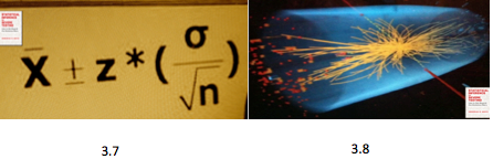
A long-standing family feud among frequentists is between hypotheses tests and confidence intervals (CIs). In fact there’s a clear duality between the two: the parameter values within the (1 – α) CI are those that are not rejectable by the corresponding test at level α. (3.7) illuminates both CIs and severity by means of this duality. A key idea is arguing from the capabilities of methods to what may be inferred. CIs thereby obtain an inferential rationale (beyond performance), and several benchmarks are reported. Continue reading
Capability and Severity: Deeper Concepts: Excerpts From Excursion 3 Tour III
Deeper Concepts 3.7, 3.8
Tour III Capability and Severity: Deeper Concepts
From the itinerary: A long-standing family feud among frequentists is between hypotheses tests and confidence intervals (CIs), but in fact there’s a clear duality between the two. The dual mission of the first stop (Section 3.7) of this tour is to illuminate both CIs and severity by means of this duality. A key idea is arguing from the capabilities of methods to what may be inferred. The severity analysis seamlessly blends testing and estimation. A typical inquiry first tests for the existence of a genuine effect and then estimates magnitudes of discrepancies, or inquires if theoretical parameter values are contained within a confidence interval. At the second stop (Section 3.8) we reopen a highly controversial matter of interpretation that is often taken as settled. It relates to statistics and the discovery of the Higgs particle – displayed in a recently opened gallery on the “Statistical Inference in Theory Testing” level of today’s museum. Continue reading
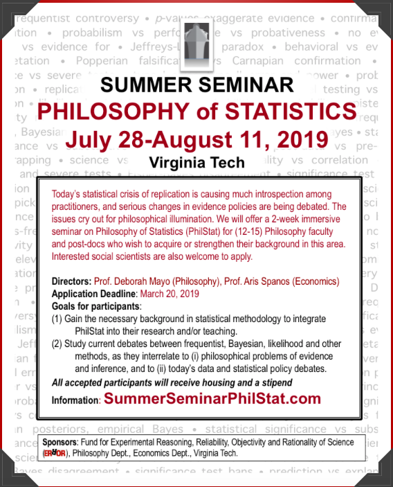
Summer Seminar PhilStat: July 28-Aug 11, 2019 (ii)
First draft of PhilStat Announcement
Mementos for “It’s the Methods, Stupid!” Excursion 3 Tour II (3.4-3.6)

some snapshots from Excursion 3 tour II.
Excursion 3 Tour II: It’s The Methods, Stupid
Tour II disentangles a jungle of conceptual issues at the heart of today’s statistics wars. The first stop (3.4) unearths the basis for a number of howlers and chestnuts thought to be licensed by Fisherian or N-P tests.* In each exhibit, we study the basis for the joke. Together, they show: the need for an adequate test statistic, the difference between implicationary (i assumptions) and actual assumptions, and the fact that tail areas serve to raise, and not lower, the bar for rejecting a null hypothesis. (Additional howlers occur in Excursion 3 Tour III)
recommended: medium to heavy shovel
It’s the Methods, Stupid: Excerpt from Excursion 3 Tour II (Mayo 2018, CUP)
 Tour II It’s the Methods, Stupid
There is perhaps in current literature a tendency to speak of the Neyman–Pearson contributions as some static system, rather than as part of the historical process of development of thought on statistical theory which is and will always go on. (Pearson 1962, 276)
This goes for Fisherian contributions as well. Unlike museums, we won’ t remain static. The lesson from Tour I of this Excursion is that Fisherian and Neyman– Pearsonian tests may be seen as offering clusters of methods appropriate for different contexts within the large taxonomy of statistical inquiries. There is an overarching pattern: Continue reading
Memento & Quiz (on SEV): Excursion 3, Tour I

.
As you enjoy the weekend discussion & concert in the Captain’s Central Limit Library & Lounge, your Tour Guide has prepared a brief overview of Excursion 3 Tour I, and a short (semi-severe) quiz on severity, based on exhibit (i).*
We move from Popper through a gallery on “Data Analysis in the 1919 Eclipse tests of the General Theory of Relativity (GTR)” (3.1) which leads to the main gallery on the origin of statistical tests (3.2) by way of a look at where the main members of our statistical cast are in 1919: Fisher, Neyman and Pearson. From the GTR episode, we identify the key elements of a statistical test–the steps in E.S. Pearson’s opening description of tests in 3.2. The classical testing notions–type I and II errors, power, consistent tests–are shown to grow out of requiring probative tests. The typical (behavioristic) formulation of N-P tests came later. The severe tester breaks out of the behavioristic prison. A first look at the severity construal of N-P tests is in Exhibit (i). Viewing statistical inference as severe testing shows how to do all N-P tests do (and more) while a member of the Fisherian Tribe (3.3). We consider the frequentist principle of evidence FEV and the divergent interpretations that are called for by Cox’s taxonomy of null hypotheses. The last member of the taxonomy–substantively based null hypotheses–returns us to the opening episode of GTR. Continue reading
First Look at N-P Methods as Severe Tests: Water plant accident [Exhibit (i) from Excursion 3]

Excursion 3 Exhibit (i)
Exhibit (i) N-P Methods as Severe Tests: First Look (Water Plant Accident)
There’s been an accident at a water plant where our ship is docked, and the cooling system had to be repaired. It is meant to ensure that the mean temperature of discharged water stays below the temperature that threatens the ecosystem, perhaps not much beyond 150 degrees Fahrenheit. There were 100 water measurements taken at randomly selected times and the sample mean x computed, each with a known standard deviation σ = 10. When the cooling system is effective, each measurement is like observing X ~ N(150, 102). Because of this variability, we expect different 100-fold water samples to lead to different values of X, but we can deduce its distribution. If each X ~N(μ = 150, 102) then X is also Normal with μ = 150, but the standard deviation of X is only σ/√n = 10/√100 = 1. So X ~ N(μ = 150, 1). Continue reading
Neyman-Pearson Tests: An Episode in Anglo-Polish Collaboration: Excerpt from Excursion 3 (3.2)
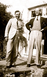
Neyman & Pearson
3.2 N-P Tests: An Episode in Anglo-Polish Collaboration*
We proceed by setting up a specific hypothesis to test, H0 in Neyman’s and my terminology, the null hypothesis in R. A. Fisher’s . . . in choosing the test, we take into account alternatives to H0 which we believe possible or at any rate consider it most important to be on the look out for . . .Three steps in constructing the test may be defined:
Step 1. We must first specify the set of results . . .
Step 2. We then divide this set by a system of ordered boundaries . . .such that as we pass across one boundary and proceed to the next, we come to a class of results which makes us more and more inclined, on the information available, to reject the hypothesis tested in favour of alternatives which differ from it by increasing amounts.
Step 3. We then, if possible, associate with each contour level the chance that, if H0 is true, a result will occur in random sampling lying beyond that level . . .
In our first papers [in 1928] we suggested that the likelihood ratio criterion, λ, was a very useful one . . . Thus Step 2 proceeded Step 3. In later papers [1933–1938] we started with a fixed value for the chance, ε, of Step 3 . . . However, although the mathematical procedure may put Step 3 before 2, we cannot put this into operation before we have decided, under Step 2, on the guiding principle to be used in choosing the contour system. That is why I have numbered the steps in this order. (Egon Pearson 1947, p. 173)
In addition to Pearson’s 1947 paper, the museum follows his account in “The Neyman–Pearson Story: 1926–34” (Pearson 1970). The subtitle is “Historical Sidelights on an Episode in Anglo-Polish Collaboration”!
We meet Jerzy Neyman at the point he’s sent to have his work sized up by Karl Pearson at University College in 1925/26. Neyman wasn’t that impressed: Continue reading

The Statistics Wars & Their Casualties

LSE PH500 Research Seminar (May 21-June 25, 2020): Controversies in Phil Stat
")
Summer Seminar 2019 (article)

Experts convene to explore new philosophy of statistics field
