
.
ANNOUNCEMENT SEV26 Synthese Topical Collection CFP: Severity and Learning from Error
This Topical Collection examines how inquiry learns from error by focusing on a basic principle of evidence in science, statistics, medicine, law, epistemology, and day-to-day learning: a claim is not well-tested, known or epistemically warranted, if it is based on a method that makes it easy to accept, conclude or infer the claim, even if it is false. Such a claim may accord well with the data, but it has not passed a stringent or severe test. While this overarching intuition is widely shared, the problem of how to understand or satisfy it remains unsolved. C. S. Peirce emphasizes randomization and (what is now called) pre-designation to achieve self-correcting methods. Popper viewed severity in terms of satisfying novel predictive success and surviving stringent attempts at falsification. Deborah Mayo (1996, 2018) combines elements from Popper and Peirce with the use of error probabilities from statistical methods: proposed solutions to problems earn warrant by surviving probes that were capable of showing them wrong or inadequate. This Topical Collection takes “severity” to be a broad meta-level concept according to which a claim – whether a report of a perception, a prediction, a hypothesis, or part of a model – is assessed according to whether, and how readily, its errors and inadequacies would have been found, if present.
Several questions arise: What errors matter for a given aim? What would it take for a method to be capable of detecting them? How in actual practice can inquirers show they have engaged in responsible error probing when there are no formal probability models? Addressing questions like these is of urgent importance today as we face high-powered methods that make it easy to find impressive looking effects that are spurious and non-replicating, or to arrive at well-fitting models that do not predict well, do not replicate, or do not provide substantive scientific understanding. These questions arise in debates about methodological shifts in AI/ML, randomized clinical trials, legal evidence, climate modeling, statistical inference, and error-prone inference in general. We seek to bring these metascience debates into direct contact and to ask what is often left hidden: What errors are now being controlled, and which have quietly dropped out of view? By bringing together philosophers, statisticians, and scientists, we aim to develop a shared set of problems and tools with a forward-looking goal: to shape emerging practices, rather than merely react to them with retrospective commentary.
We welcome submissions on any topic that broadly relates to severity or learning from error. We invite contributions that develop, apply or challenge severity-based reasoning, or that develop alternative approaches, Bayesian, frequentist, machine-learning and other, which engage the same underlying concern: how inquiry learns from error, and how claims earn warrant by surviving probes that were capable of showing them wrong or inadequate. We encourage contributions that explore connections between concepts of severity in different fields. Notably, the concepts of sensitivity and safety in contemporary epistemology can be understood through the lens of severity, and both are redolent of stability in AI. We also welcome discussions of how contemporary manifestations of severity interrelate with the traditional notions of severity from Popper and Peirce, and how concepts of severity may help in tackling fundamental problems of induction, falsification, underdetermination, and realism in philosophy of science.
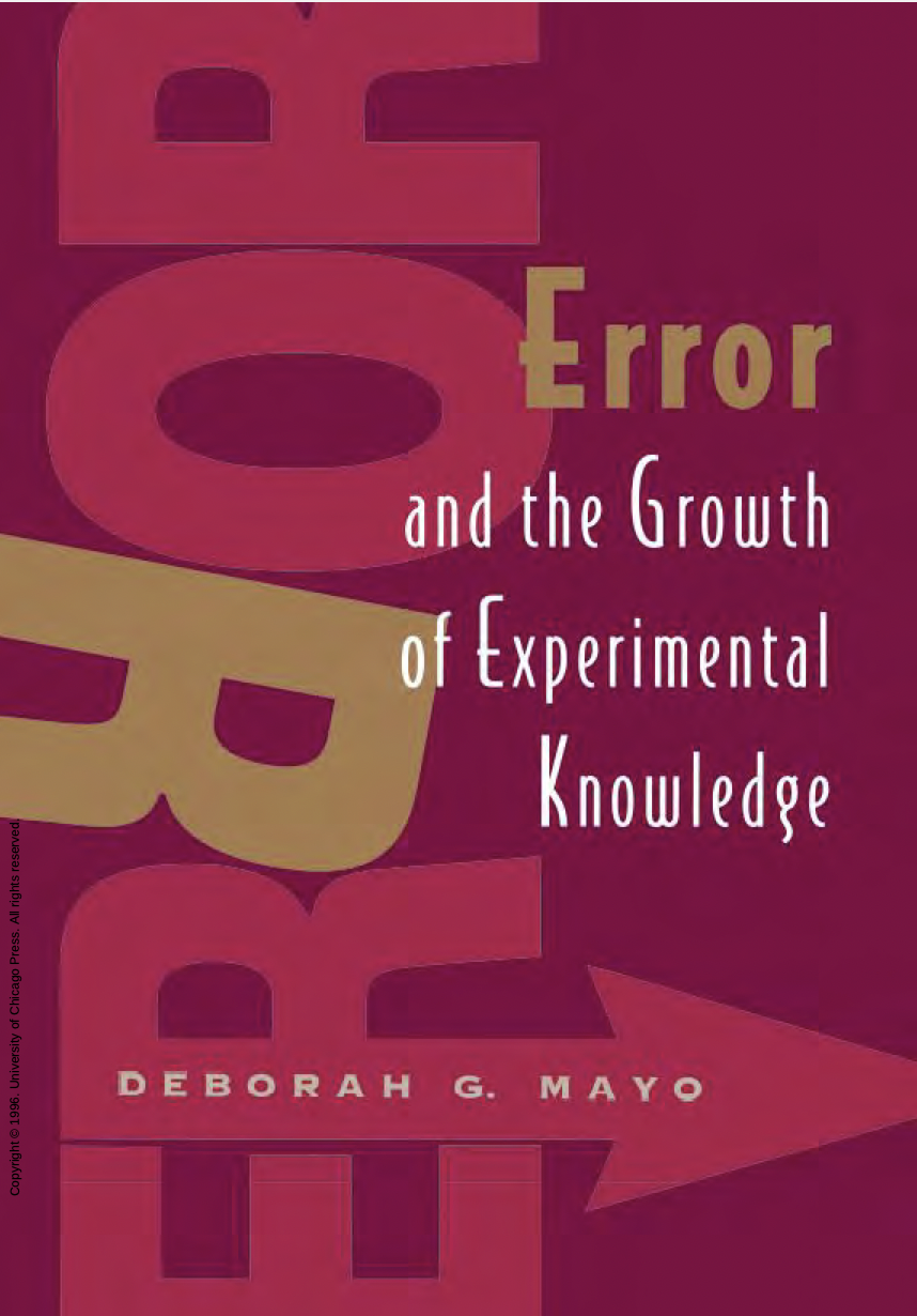
The collection is partly motivated by the thirtieth anniversary of Deborah Mayo’s (1996, Chicago) Error and the Growth of Experimental Knowledge (Lakatos Prize 1998) and the development of its account of severe testing.
Appropriate Topics for Submission include, among others:
Severity and philosophy of statistics
- Do recent controversies about the uses of error probabilities in statistics (and metastatistics) present a challenge to severity-based reasoning?
- Do the new fields of post-selection inference (in AI and other disciplines) allow for error control despite data-driven constructions? Or do they shift attention to different errors?
- How does severity link to such notions as calibration, security, and stability, and statistical techniques that promote such notions as robustness analyses, and multiverse analyses?
Severity and philosophy of science
- What does it mean for a method, or for science itself, to be self-correcting or error-correcting? Does it fit best with a pragmatist philosophy?
- How does severe probing take place in the historical sciences, e.g., climate science, geology? Can claims be well probed without being replicable?
- Rather than probing for falsity, how can we severely probe if a model is adequate for a purpose or problem of interest?
Severity and contemporary epistemology
- Can a useful cross-cutting epistemology that links science, statistics, and applied epistemology be built around the concept of severity?
- Do features of severity (e.g., auditing of assumptions) point to ways to avoid problems of sensitivity and safety in epistemology?
- Does requiring severity explain why legal epistemology resists mere base-rates and “naked statistics”? Does it solve proof paradoxes in legal epistemology?
Tracking shifts in error control
- How does AI/ML shift from modeling data-generating mechanisms in statistics to optimizing predictive performance in machine learning.
- How do changing guidelines for RCTs shift trials from probing biological mechanisms to predicting average treatment effects over a population?
- What are the social, epistemic, ethical, and political consequences of shifting regimens of error control?
The value of probing error
- How can adversarial collaborations and stress-testing advance science?
- How can error repertoires be built and effectively employed to facilitate severity in measurement and experiment?
- How does learning from error enter outside science (e.g., in art, architecture and life drawing)?
Submissions via: https://www.editorialmanager.com/synt/default.aspx
Under the drop-down menu, select Severity and Learning from Error.
Submitted papers will undergo the usual Synthese review process.
For further information, please contact the guest editors:
mayod@vt.edu, wendyparker@vt.edu, D.Lakens@tue.nl, staleykw@gmail.com.
The deadline for submissions is the 15th of December, 2026 (with possible short extensions). Use the comments or write to me with your ideas and questions with the subject: SEV26. The website announcement is here: https://link.springer.com/collections/ebjdhfadcd


 The concept of a test’s power, originating in Neyman-Pearson’s early work, by and large, is a pre-data concept for purposes of specifying a test (notably, determining worthwhile sample size), and choosing between tests. In some papers, however, Neyman lists a third goal for power: to interpret test results post data much in the spirit of what is often called “power analysis”. This is to determine the discrepancy from a null hypothesis that may be ruled out, given nonsignificant results. One example is in a paper “


")

