

.
Stephen Senn
Consultant Statistician
Edinburgh
Relevant significance?
Be careful what you wish for
Despised and Rejected
Scarcely a good word can be had for statistical significance these days. We are admonished (as if we did not know) that just because a null hypothesis has been ‘rejected’ by some statistical test, it does not mean it is not true and thus it does not follow that significance implies a genuine effect of treatment.
However, it gets worse. Even if a hypothesis is rejected and the effect is assumed genuine, it does not mean it is important. For those of you, who like me, haunt the statistical discussion pages of LinkedIn, very few days seem to pass before you get an automated notification to read some blog lecturing you about the dangers of confusing statistical significance and clinical relevance. This too, I think, is something we knew.
You ain’t seen nothing yet
However, you should be very careful about what you are going to demand from clinical trials. If you think that statistical significance is a slippery concept, clinical relevance is even worse. For example, many a distinguished commentator on clinical trials has confused the difference you would be happy to find with the difference you would not like to miss. The former is smaller than the latter. For reasons I have explained in this blog (reblogged here), you should use the latter for determining the sample size as part of a conventional power calculation.
In what follows, I shall distinguish these two concepts as follows. I shall use the symbol δ1 to mean the difference we should be happy to find and the symbol δ4 to mean the difference we should not like to miss. The reason I have chosen subscripts 1 and 4 is that in terms of my previous blog, δ1 is the first of the four possible meanings of clinically relevant and δ4 is the fourth. I shall also make the simplifying assumption that we can measure treatment effects so that positive values are ‘good’. That being so, we have δ1< δ4.
One out of two ain’t bad
Now suppose that we are going to plan a clinical trial for an indication in which we have (just to make things simple) δ4 = 1 for an outcome that we assume to be Normally distributed. Now suppose that we plan to have a conventional two-sided test at the 5% level, that is to say, with α = 0.05 (to use the conventional symbol). Suppose, furthermore, that we should like to have 80% power, that is to say β = 0.2 (continuing the same symbolic convention) for the case when the ‘true’ value of the treatment effect is exactly equal to δ4. Ignoring a refinement involving the non-central t-distribution, we can proceed approximately as follows.
-
- We note that a value of 1.96 for the standard Normal corresponds to a tail area probability of 2.5%, or α/2 = 0.025.
- We note that a value of 0.84 for the standard Normal corresponds to a tail area probability of β=0.2, which would give us 80% power.
- The sum of these two values is 1.96 + 0.84 = 2.8.
- We now need to plan for a sample size that will deliver a standard error (SE) that will yield δ4/SE = 2.8 that is to say SE = δ4/2.8 .
- Since δ4 = 1, we thus require a sample size that gives SE = 1/2.8 = 0.357.
There are of course a number of difficulties with this. For example, although the SE is a function of the sample size and the allocation ratio (treatment to control), both of which we can determine, it is also a function of the standard deviation of the measurements, of which, since at the time of planning, the measurements lie in the future, we can only have informed guesses. Nevertheless, this description is sufficient to show the problem.
Picture this
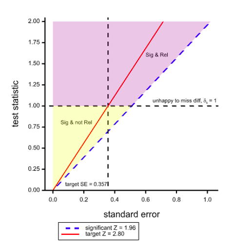
Figure 1. Two dimensional space with the test statistic on the Y axis and its SE on the X axis showing boundaries for regions of statistical significance and clinical relevance.
Figure 1 shows a space that covers pairs of values of the standard error (the X dimension) and the test statistic (the Y dimension). The dashed diagonal line is the line of ‘minimal significance’. Along this line the ratio of statistic to SE is 1.96 which will just yield significance at the 5% level, two-sided. It thus follows that any (SE, statistic) point to the left of and above this line is statistically significant. The red line corresponds to the target ratio of 2.8 that is supposed to deliver 80% power for 5% significance.
However, if we take the value of δ4 = 1 used for planning the trial as defining clinical relevance and we add the further requirement for success that the point estimate should also be equal to δ4 as well as the results being statistically significant, then the horizontal dashed line divides the significant region into two: the purple part above the line where the point estimate is also ‘clinically relevant’ using this (unwise) standard and the yellow region below where it is not. The net result of such a requirement would be that even if the SE turns out to be exactly as planned, ‘power’, if one may term the joint requirement thus, will not be 80% as planned but only 50%.
Note that this applies a fortiori if we make the further requirement that not only should we observe a clinically relevant difference, that is to say obtain a point estimate at least as great as this, but we should ‘prove’ that it obtains, for example by obtaining a confidence interval that excludes any inferior values.
We can work it out
What is the solution? The only possible solution is to use a definition of clinical relevance for judging practically the acceptability of a trial result that is more modest than that used for the power calculation. If we set δ1 = 0.7 in the above case (shown by the lower horizontal dashed line), then if the SE is as planned and hoped for, we have the consequence that a significant result is a clinically relevant one. Thus the 80% power is maintained, at least for this planned case. This situation is illustrated in Figure 2, where a part of the region that was previously yellow and designated as significant but not relevant is now orange and can be added to the purple region.
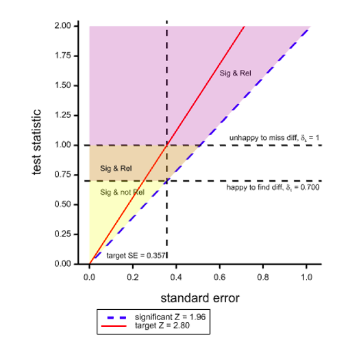
Figure 2. Situation as illustrated before but with a less ambitious target of δ1 for ‘clinical relevance’
Ironically, using this standard, the only way we can obtain a significant result that is not ‘clinically relevant’ is if the SE is lower than planned. If the SE is higher than planned, we shall have affected power badly but we shall not have significant results that are not ‘relevant’.
Note, of course, as discussed above, this is a standard for observing a clinically relevant difference. It would be naïve to assume that, just because we have (a) ‘rejected’ a null hypothesis and (b) observed a clinically relevant difference, we can therefore conclude that the difference is necessarily that observed. However, pursuing that particular line of thought introduces further complications it is not necessary to examine in order to show that one should be very cautious about making requirements for clinical relevance. Some commentators have already found the requirement for conventional power excessive (Feinstein and Concato 1998).
I can see clearly now
Well, we can see clearly, at least, that it’s all very well lecturing the world about requiring clinical relevance but you need to do more than that and clarify what exactly it is that you are asking for. My advice is, ‘be careful’.
Acknowledgement
I am grateful to Deborah Mayo for helpful comments on an earlier version. Any errors that remain are my own.
Reference
R. Feinstein and J. Concato (1998) The quest for “power”: contradictory hypotheses and inflated sample sizes. Journal of clinical epidemiology, 537-545.
Invite readers to share remarks and questions in the comments.


")


Stephen:
I’m extremely grateful to you for all of the interesting and provocative posts you’ve contributed to this blog. I will write a distinct comment shortly.
Thank you!
Mayo
Stephen:
I very much appreciate this post because it helps to illuminate an issue that seems increasingly confused. In particular, I want to emphasize your point that “It would be naïve to assume that, just because we have (a) ‘rejected’ a null hypothesis and (b) observed a clinically relevant difference, we can therefore conclude that the difference is necessarily that observed.” I would even propose strengthening it by alluding to your remark about confidence intervals. In other words, just because we have observed a clinically relevant difference, we cannot infer evidence the population or parametric difference is as large as what’s observed. This would require, as you say, “obtaining a confidence interval that excludes any inferior values”. For the confidence level to be reasonable high, one would need to subtract, say, 1.6 SE, from the observed difference. You explain all this in your book Statistical Issues in Drug Development (e.g., 13.2.4).
When we run, say, a 1-sided positive test, it seems to me, we’re “happy to be alerted to” any genuine positive discrepancy from the reference value chosen for the null hypothesis. Ascertaining the discrepancies well (or poorly) warranted would be a distinct step, either via confidence intervals, a severity assessment, or considering a series of p-values for different discrepancies.
You are right that statistical significance tests are “rejected and despised” by some, but I would say that they remain the only game in town when it comes to the job of testing if there’s a genuine discrepancy from a reference value or model–whether it’s an ordinary p-value or perhaps a falsificationist Bayesian p-value (Gelman). Neither Bayes factors nor posterior probabilities can provide such tests–unless they’re supplemented with frequentist error probabilities (which is futuristic). It is noteworthy that Berger, Bernardo and Sun do not include statistical tests in their Objective Bayesian Inference (2024)–not even Bayes factors. When AI/ML researchers wish to evaluate and compare algorithms, and in developments in “selective inference,” standard error probability criteria are central.
Very interesting, thank you.
Could that be an argument for the value of well-conducted systematic reviews and meta-analyses of trials designed to detect delta4 with the aim of detecting delta1?
Stephen, this is fantastic, thanks for this! It’s an argument that I’ve had with folks often, back in the past when I used to do clinical research. That said, I do have 2 minor quibbles with your notation. First, you labeled your Y-axes “test statistic”, and it took me a bit to understand that there you just meant the unscaled difference, i.e., the delta. Then, in Figure 2, you stuck with delta 1 for the “happy to find” diff, while you had called that delta 4 previously. And, of course, I’m left wondering about delta 2 and delta 3, but I guess I just have to read, or re-read possibly, the original blog post.
Glad to see that Mayo is still hosting excellent discussions!
Mark:
I placed that earlier blogpost here:
I’m about to post a comment on it.
Mark and Stephen:
I see Mark’s point now and the switch Stephen makes in clinically relevant. He says, “The only possible solution is to use a definition of clinical relevance for judging practically the acceptability of a trial result that is more modest than that used for the power calculation. If we set δ1 = 0.7 in the above case (shown by the lower horizontal dashed line), then if the SE is as planned and hoped for, we have the consequence that a significant result is a clinically relevant one. Thus the 80% power is maintained, at least for this planned case.”
80% power is maintained for ….delta-4. If delta-1 is now the clinically relevant difference, set equal to the observed difference that is just statistically significant, then we’re back to 50% power associated with delta-1. I had initially assumed clinical relevance was always to be viewed as the (population) difference we would not wish to miss (delta-4)–the highly relevant difference– while introducing delta-1 as a difference of practical interest, a difference happy to find, or the like. Stephen can clarify. The 4 deltas in the previous post were:
1.It is the difference we would like to observe
2. It is the difference we would like to ‘prove’ obtains
3. It is the difference we believe obtains
4. It is the difference you would not like to miss.
My main concern is that construing a (just) statistically significant difference as clinically relevant makes it sound as if it’s evidence for a clinically relevant difference, whereas, in fact, as Senn notes, it’s only good evidence that the underlying difference exceeds the lower confidence bound (at a reasonable level). (I would not use prove.) This is assuming a just statistically significant difference is observed.
Stephen:
A major source of perplexing construals of power is the tendency among Bayesians to view it as a likelihood or conditional probability. Say there is high power associated with delta. Since I don’t know how to write Greek symbols in comments, I’ll write it as d. The Bayesian reasoning goes like this:
If the population effect size is d, then there’s high probability of the test rejecting the null hypothesis (i.e., the power associated with d is high)
The test rejects the null hypothesis.
Therefore, it is evidence of a population effect size d.
This is probabilistic affirming the consequent. The consequence of this is that the more discrepant the alternative considered (and thus, the higher the power), the stronger the evidence it is accorded by a rejection of the null at a given level—which is backwards, at least for error statistical testers or confidence interval users..
I’ve discussed this a few times on this blog, such as here:
https://errorstatistics.com/2016/04/11/when-the-rejection-ratio-1-βα-turns-evidence-on-its-head-for-those-practicing-in-the-error-statistical-tribe/ Bayarri, Benjamin
I don’t see how delta-3 in your previous blogpost can make sense. I know you reject it, but how can even Bayesians accept it? As I understand it, the clinically relevant difference is some (population) effect size deemed of interest, say an increase in progression-free survival of a year. Yes? It would seem to lead to always believing the clinically relevant difference obtains.
Peter:
This remark made me go back to Senn’s earlier post and what the different delta’s are. That led to my response to Mark. You’re right that it would be peculiar to choose delta-3, but it’s actually behind a lot of criticisms of p-values, as in “redefine significance” (Benjamin et al 2018). It take it the idea is that this is the value believed under the alternative. We did discuss this in the seminar.
Thanks, for hosting these two blogs Deborah. I think that the general point I have tried to make is that if you design a clinical trial to have a particular desired operating characteristic, you should be careful about assuming that it will deliver others.
As it happens, I am not a great fan of conventional power calculations because the extremely important element of cost, whether measured in money or human suffering is missing. Nevertheless, I do regard the conditional nature of a power calculation as reasonable. It’s reasonable to set up a procedure to make it probable that you would flag a drug that is interesting while controlling the probability of declaring a completely useless drug effective.
However, there is a big range between these two extremes and this is where the problem arises. What I was pointing out in the blogs is that you can’t expect that the system will do more than it has been designed to do. Furthermore you cannot get it to do more without investing more resources. You may then find that ethical and practical difficulties set in.
The way I used to think about it when I worked (directly) in drug development is this. If the trial stops and we don’t declare the lead worth pursuing we will never study the drug again. If we do decide to pursue the lead, more information will accrue and we can refine our opinion. Thus it makes sense to choose a delta that you would not like to miss.
Furthermore, what you are operating is a system for screening candidates. The test is to that extent independent of what we may believe about the candidate. Given this perspective, delta is a quality of the disease. Assurance seeks to make it a quality of the drug. This, I think, is a mistake.
However, the main point is that if you demand not only statistical significance but also clinical relevance, you may be disappointed to find that you get the former but not the latter, especially if you make the mistake of confusing delta 4 and delta 1,
Thank you so much for your guestpost and comment. I have a confusion and a concern. I think what’s confusing me is what you recommend as opposed to what you entertain (to show people what can happen if they get what they wished for). I assumed at first, and now again I’ve come back to this, that you were retaining the same view as before, in the previous post and your book, that delta is the clinically relevant difference construed as:
“the difference you would not like to miss”
or, equivalently,
“the difference you would be unhappy to miss”.
Then, yesterday I thought you might be changing it to delta-1, because Figure 2 says delta-1 is clinical relevance. This was, I took it, a way to make significance tests more palatable to its critics. By allowing it to be delta-1, the difference we would like to observe, it follows that observing a statistically significant difference is now to observe a clinically relevant difference. A clinically relevant difference is now one that the tester “would be happy to find”.
My concern is that people will then understand “a significant result is a clinically relevant one” to mean a (just) statistically significant difference is evidence of a clinically relevant difference. And that would be incorrect. Moreover, the result might just be reported as statistically significant at the alpha level. Of course, even N-P recommended looking at the attained p-value. But the attained p-value for the hypothesis: “the population difference equals the observed difference” would be .5. So even with the less ambitious delta-1 for clinical relevance, testers would need to be aware that observing a clinically relevant difference was not evidence of a clinically relevant difference. (Won’t they be unhappy to find this out? I know you say it doesn’t “prove” it, but what about “strong evidence”?)
Another thing I’d be grateful for clarification on: I thought the clinically relevant difference, in your view, was essentially fixed, based on substantive knowledge. Is that correct? Perhaps the less ambitious clinically relevant difference, delta-1, should be construed as something like “minimally (or moderately) clinically relevant”, and delta-4 is “highly clinically relevant”? Is that the idea?
Anyway, today I am thinking that you are largely illustrating a way to have high power for a “(highly) clinically significant difference” delta-4 while still being able to take a just statistically significant difference as at least moderately clinically relevant—rather than recommending testers do this. But it would still be wrong to take a (just) statistically significant difference as evidence of a moderately clinically relevant difference. It would only be evidence for a difference greater than the lower confidence bound, at a reasonable level. That, of course, is what the N-P test provides: A just statistically significant difference is evidence that the population difference exceeds 0 (for this type of null). Larger observed differences enables larger inferred effect sizes. I use “discrepancy” for population effect sizes. My view is that testers are happy to find strong evidence for any genuine discrepancy from Ho—that’s to falsify (statistically) the null. Warranted discrepancies can be separately ascertained.
I’m sorry this got so long, but can you say what your recommendation is? The last paragraph of your comment, about choosing a delta you would not like to miss, is still a bit cryptic. Is that equal to one you’d require high power to detect = clinically significant.?
My apologies for not being clear. The problem is that clinically relevant difference can mean so many different things.
If you want it to be the value you would like to use for a power calculation, then it has to be delta 4. If I used a conventional power calculation to determine a sample size i would always always try and get some understanding as to what the client thought a delta 4 type value would be.
If you want the clinical relevant difference to be a value you would be happy to observe (with the understanding that just because you observed something it does not have to be “true”) then you need to talk in terms of delta 1. You should not use this to carry out a power calculation.
Delta 3 is the difference you (or somebody) believes obtains and, of course, it requires a distribution. The only use for this is to decide whether a trial is worth doing at all. It is a bad idea, in my opinion, to use it to guide the sample size. This would have the effect of directing you to use more resources whenever you believe the effect is small and if that belief itself has any value, this would be perverse, bearing mind that there are other drugs projects for resources.
It only makes sense if a choice must be made between A and B (and there is no C,D, E etc waiting and no realistic prospect of finding them) and the population of potential patients is very large compared to those available for study.
I don’t think that delta 3 makes sense either except in the following circumstances.
You believe that the treatment works and your expected value for the effect is delta 3.
You want to convince others who don’t share your belief.
They can be convinced by a conventionally “significant result”.
You want to calculate the probability that you will succeed in objective 3 given the details (including sample size) of the trial you are going to run.
Where that is the case, something like assurance an idea proposed by O’Hagan and Stevens about 25 years ago may be useful. See, for example, Assurance in clinical trial design – O’Hagan – 2005 – Pharmaceutical Statistics – Wiley Online Library.
It is also useful to correct the (obviously false but sometimes falsely held) notion that power is the probability of “success”. In my opinion it is not a good idea to try and adjust the sample size to boost the value of assurance, for reason explained in section 13.2.16 of Statistical Issues in Drug Development, 3rd Edition, 2021
Apologies. I am finding it difficult to handle WordPress, which, it seems, no longer allows me to log-in as a guest and has given me a bizarre username.
A previous reply to Deborah Mayo has also disappeared down some internet black hole.
Stephen Senn
Stephen:
I’m sorry, I’ve no clue where that name came from (I’ve corrected it) but I recall this happening once before. Can you please resend the comment that went down the black hole? I’m checking the site.
Mayo
Dear Dr. Senn,
Thank you for these valuable clarifications regarding some of the hidden risks embedded within the often vague notion of “clinical relevance” in statistical discourse. In this regard, I would like to take inspiration from your reflections to highlight a few related issues, which I believe are sometimes misused to justify methods not grounded in a robust body of literature. In my view, your recommendation to adopt more lenient criteria deserves to be extended well beyond the context discussed here, in order to avoid reducing statistics to a set of mathematically coherent procedures built upon assumptions that are often unrealistic or unverifiable in real-world settings.
To the best of my knowledge, the concepts of power and statistical significance linked to the decision thresholds α and β in the Neyman-Pearson framework are operationally meaningful only in the context of high volumes of decisions – such as those involving multiple independent hypotheses within a single study or the same hypothesis tested across many replication attempts – and only when errors are predominantly random, approximately following an ideal distribution or law, and the true effect is sufficiently stable or governed by well-specified laws. The reality I observe is largely incompatible with these premises. For instance, a recent study by van Zwet et al. shows how – under plausible conditions – the above assumptions are substantially violated even in a collection of over 23,000 randomized trials [1], which are arguably the most ideal experiments we can realize in practice. This aligns with the well-documented issues of transportability and generalizability [2], as well as academic distortions [3] and rituals [4].
Secondly, and no less importantly, the very concept of a cost-benefit ratio may be a gross oversimplification of real-world complexity (a point of criticism I also direct at my own work). Proper decision-making requires assessing multiple layers of highly contextual advantages and disadvantages, often evaluated according to criteria that are deeply shaped by subjective interpretations rather than being reducible to a single unified endpoint. The binary “effective vs. ineffective” (or even the softened version “more effective vs. less effective”) also fails to capture the inherently multivariate nature of outcomes in therapies and interventions. These are often characterized by heterogeneous side effects (e.g., varying in intensity, type, frequency, duration, or triggering factors), costs that depend heavily on how endpoints are defined (e.g., short-term vs. long-term financial impact), and benefits that similarly vary depending on the chosen objectives – such as maximizing survival, enhancing quality of life, or balancing competing priorities – and the strategies deemed appropriate to pursue them.
With respect to these latter points, it is crucial to acknowledge the high degrees of subjectivity and context-dependence involved in defining endpoints [5], even multivariate ones. Such variability cannot be meaningfully condensed into a single hypothesis (not even when expressed as a multivariate vector, which is rare in my experience) to be tested through a dichotomous decision rule. Indeed, even at the purely statistical level, there are striking examples that illustrate how such precision is generally unattainable [1]. On this basis, methods often mystified as definitive solutions, such as equivalence testing, appear to me more as wishful thinking at best, even setting aside their internal consistency issues as discussed by Greenland and others before him [6,7]. Ultimately, every cost-benefit assessment rests on complex ethical considerations (e.g., should we prioritize transplanting a younger patient with better odds of survival even without the transplant but a potentially higher benefit, or an older patient in the opposite scenario?) and contextual conditions (e.g., the effectiveness and objectives of a vaccination strategy depend on the broader epidemiological landscape, including viral or bacterial mutations, lifestyle changes, shifts in health behavior and the healthcare system itself). Hence, I find the ambition to condense all such information into a single testable hypothesis both arbitrary and intellectually presumptuous.
Many argue that a threshold is needed to make the decision rule objective or impartial. But as Neyman himself clearly stated in a 1977 paper, the establishment of any threshold inevitably involves a strong subjective component [8]. Thus, we are not avoiding value-laden discussions but embedding them in a complex mathematical framework, i.e., we are merely concealing them. This, combined with the mathematical-statistical intricacies of the models (e.g., in Cox models, those related to collapsibility, events per variables, hazards proportionality, etc.), further complicates our overall ability to assess how analytical priors mechanically influence or shape healthcare decisions.
Therefore, I would advocate for adopting unconditional descriptive frameworks, even in studies labeled as confirmatory, since robust causal inference may require decades to be established properly in many fields or subfields of medicine. In my opinion, the goal of scientific studies should be to summarize the available information while limiting the impact of priors and making such priors explicit – both mathematically and methodologically – as far as possible. It is then up to regulatory bodies to make regulatory decisions, continuously monitoring how well real-world data agree with those decisions over time, context by context.
Of course, I would be very interested to hear your thoughts on these reflections and look forward to any comments you might wish to share.
All the Best,
Alessandro
REFERENCES
1. https://doi.org/10.1056/EVIDoa2300003
2. https://doi.org/10.1007/s10654-023-01067-4
3. https://doi.org/10.1093/ije/dyad181
4. https://doi.org/10.1177/2515245918771329
5. https://doi.org/10.1136/jech-2011-200459
6. https://doi.org/10.1111/sjos.12625
7. https://doi.org/10.1214/ss/1032280304
8. https://doi.org/10.1007/BF00485695
Thanks. I can agree with a number of these points but not all.
For example, I am not sure that Van Zwet et al can be interpreted in the way that you suggest. I consider that my blog proposed the following.
One interpretation of their results is that delta 3 is less than delta 4. I see no problem with this even if i see value in statisticians and others being reminded by this sort of study of the regression effect.
I don’t accept that analysis of trials should be descriptive.
I do find the possibility of looking at outcomes in a multivariate sense intriguing and potentially valuable. I have only thought about this occasionally from time to time and must confess that I have no practical suggestion as to how one should proceed.
Dear Dr. Senn,
Thank you for your response. I’m glad to find areas of agreement between us, and I’d like to further clarify some points where we may differ.
Regarding the study by van Zwet et al., I agree that their results are less concerning within your more relaxed framework (which I support in its philosophy) and are coherent with some decision rules. However, the key underlying issue is the meaning of such rules. For instance, if the rule follows the widespread convention of setting α=0.05 and β=0.90 (or 0.80), then it arguably contradicts Neyman’s own requirement that thresholds be established based on contextual relevance [1, p.103]. In this regard, as Neyman emphasized, both the definition of success and the method used to evaluate it are subjective and external to mathematics [1, pp.99-100]. To take a more moderate stance, I believe we can agree that these elements involve at least a substantial degree of subjectivity.
Conversely, if we assume that each (α, β) pair has been chosen with careful attention to context, then the issue becomes precisely the impact of subjective choices, including those shaped by limited knowledge of a constantly evolving, complex context. Among other consequences, this uncertainty can plausibly give rise to non-random errors, which can undermine the expectation that type I and type II errors will converge toward the arithmetic mean of various α₁,…,αₙ and β₁,…,βₙ across studies [1, pp.108-109]. More fundamentally, however, I see a broader issue: the likely lack of representativeness of the target hypothesis with respect to the actual endpoint – which, as I believe you would agree, is generally multivariate and highly situational. Here too, the default choice of the null hypothesis is a ritualistic act, in contrast with Neyman’s explicit insistence that hypothesis formulation be grounded in contextual relevance [1, pp. 106-107]. In addition, this approach becomes particularly problematic in light of the strong assumptions that must hold – both statistically and causally – for such a hypothesis to be appropriate given the scientific goal, and relative to the chosen α and β [2-4]. In this regard, information about any cost-benefit ratio may only become clear after a long time, as may the degree of exchangeability, generalizability, and transportability [4]. Finally, beyond common forms of selection and information bias, as well as issues related to study design [4], we cannot ignore the fact that those who have the resources to conduct large-scale trials (or studies in general) often coincide with those who have a vested interest in obtaining results in a specific direction. In such cases, it is easy to choose α and β based on estimated convenience, and only afterward construct a rationale to justify those choices.
In this light, I’d like to propose a possible middle ground: wouldn’t it be reasonable for authors to first report their results in the most descriptive and transparent way possible – thus allowing for a more “independent” or at least “less prior-conditioned” interpretation – and only afterward, in a separate section, present their own decision framework and the results strongly conditional on that approach? In other words, don’t you think what we truly need is fewer claims of significance or non-significance by authors – often shaped in intricate ways by their own choices and beliefs – and more studies that provide clearer, broadly interpretable information [5]?
I do understand your position on not accepting a purely descriptive stance in the analysis of clinical trials; nonetheless, given the above points, I still find it difficult to provide a robust justification for any prescriptive rule of behavior, although I agree that your distinction between the various δᵢ is a meaningful and constructive step in the right direction.
All the Best,
Alessandro
REFERENCES
1. doi: 10.1007/BF00485695
2. doi: 10.1080/00031305.2018.1527253
3. doi: 10.1145/3501714.3501747
4. doi: 10.1007/s10654-019-00533-2
5. doi: 10.48550/arXiv.1909.08583
Alessandro:
Just to give my opinion of your “middle ground”. The recommendation that authors merely “describe” their results, imagining it’s being done in the most “transparent way possible” would reward those most skilled in salesmanship—those adept at appearing transparent while subtly shaping interpretation to fit the vested interests you mention. The better one is at spin, the higher the salary.
Being “external to mathematics” scarcely makes error statistical choices immune from objective criticism. On the contrary, Neyman and Pearson saw them as necessary for critical testing. In their view, the ability to interpret statistical results is inseparable from how the experiment was designed and how hypotheses were chosen for testing. If one plans to report findings without reference to error probabilities, there’s little incentive for those design principles to enter at the start. By the time the author’s favored construal of the results is in, it’s too late to recover the inferential constraints they would have provided.
Let’s see what Senn says.
Dear Dr. Mayo,
Far be it from me to suggest a simple solution to a complex and multifaceted problem. Nonetheless, the descriptive approach is grounded, first and foremost, in an aspect that stands apart from encapsulating narratives – including causal explanations – which can be distorted by rhetorical skill and other psychological influences. Perhaps the best way to describe it is as an extension of descriptive statistics. For example, authors simply report and/or summarize the results as they are, without applying hard decision rules or adjustments for multiple comparisons – unless such adjustments are presented explicitly as part of a sensitivity analysis.
I’m not claiming that this practice is immune to distortion. However, if such distortions arise at this basic level, they are likely to have an even greater impact on subsequent layers of analysis that inevitably rest upon that descriptive foundation. For instance, any declaration of significance is necessarily preceded by an initial descriptive analysis in the sense just described.
Secondly, the unconditional descriptive approach follows a clear and specific protocol. Conceptually, it could be simplified to the principle that limitations of the analysis should be presented alongside the main results – including in summary sections such as the abstract and conclusion. This is something that can be easily checked during peer review, since it amounts to ensuring that the “limitations” section is not relegated to a hidden corner of the paper, but instead integrated into the most communicatively impactful parts of the article, giving equal cognitive weight and legitimacy to all hypotheses compatible with the data scenario. In this regard, it may be necessary to reconsider the very notion of “limitations” and instead frame them as “alternative hypotheses compatible with the data” – that is, possible phenomena that could explain the observed and/or computed numbers. From a scientific standpoint, these possible phenomena are – and should be treated as – equally important as the target hypothesis.
Even conceding, for the sake of argument, that the unconditional descriptive approach is not part of the solution, I still fail to see how the Neyman-Pearson framework could address the issues raised above in real-world contexts. Indeed, the assumptions on which that framework relies are frequently and seriously violated – problems such as lack of randomization, exchangeability, or representativeness are very common, especially in certain areas of medicine. This includes the almost universally overlooked requirement for a high volume of decisions to properly implement its inferential logic under strictly ideal (if not utopian) conditions.
Best,
Alessandro
Maybe. As I often say, we are moving from an era of privately held data and a single shared analysis, to publicly shared data and a myriad of analyses. This seems to be the essence of the internet. I remain profoundly pessimistic, however, that this will improve the quality of debate. Pre-specified and registered analyses are the norm in drug development and post-hoc rationalisation the province of academia (a field, since you raise vested interests, that regularly provides material for Retraction Watch). I have my doubts that increasing the scope for post-hoc analyses is a good idea.
Dear Dr. Senn,
I very much agree with your “maybe.” As I mentioned earlier to Dr. Mayo, I do not claim to have a magic solution to a problem that is both complex and difficult to fully grasp. I also strongly agree with your point about information overload, which has become a major and growing concern not only within the scientific community, especially in the post-COVID-19 era.
We clearly operate within a network of trust, in which many important decisions are made on our behalf by others. Often, we are not even aware that these decisions are being made. My aim is simply to ensure that those entrusted with this responsibility – who, in an ideal world, would be the most knowledgeable individuals on the matter – are equipped with the means to perform independent analyses effectively and with minimal friction.
One of the major unknowns in this regard is the role of artificial intelligence, which could greatly simplify many components of this challenge while simultaneously amplifying others through the integration of human biases [1,2], prognostic capabilities hidden within so-called black boxes [3], and large disparities in access and computational power driven by socioeconomic inequality.
Given this complex landscape, I believe that at least one of the goals of the unconditional compatibility approach is both realistic and important: namely, to ensure that all identified hypotheses compatible with the presented data are featured in the summary sections (which carry greater communicative weight), rather than being relegated to the often-overlooked “limitations” section. This simple step could be crucial in beginning to assign appropriate cognitive weight to what are now merely “currently [cognitively] subordinate factors” [4].
Best,
Alessandro
REFERENCES
Stephen:
Your post illuminates another connection between power and what is shown by statistical significance test results: nonsignificant results. If a test with high power to detect delta-4 yields a statistically insignificant result, it is evidence the (population) effect size is less than delta-4. (Were it as great as delta-4, then with high probability we would have observed a larger difference.) Note too how this relates to the corresponding upper confidence bound, using a just insignificant result (i.e., one that just misses the cut-off for significance).
Neyman developed confidence intervals, and also connected it to power. In his “The Problem of Inductive Inference” (1955) Neyman criticizes Carnap:
“I am concerned with the term ‘degree of confirmation’ introduced by Carnap . . .We have seen that the application of the locally best one-sided test to the data . . .failed to reject the hypothesis [that the n observations come from a source in which the null hypothesis is true]. The question is: does this result ‘confirm’ the hypothesis [that H0 is true of the particular data set]?” (p. 40)
“The answer . . . depends very much on the exact meaning given to the words ‘confirmation,’ ‘confidence,’ etc. If one uses these words to describe one’s intuitive feeling of confidence in the hypothesis tested H0, then . . . the attitude described is dangerous . . . the chance of detecting the presence [of discrepancy from the null], when only [n] observations are available, is extremely slim, even if [the discrepancy is present]. Therefore, the failure of the test to reject H0 cannot be reasonably considered as anything like a confirmation of H0. The situation would have been radically different if the power function [corresponding to a discrepancy of interest] were, for example, greater than 0.95.” (p. 41)
Neyman shows that power analysis uses the same reasoning as does significance testing. Using (what I call) attained power and severity, a more nuanced assessment of the discrepancies well or poorly warranted emerges. “This avoids unwarranted interpretations of consistency with H0 with insensitive tests . . . [and] is more relevant to specific data than is the notion of power” (Mayo and Cox [2006], p. 89)
I am interested in the statistical significance de-testers you mention at the start of your post. (May 28: I notice you wrote “despised” but “detested” fits better.) As an outsider, I am much less aware of the current statistics wars than you. Critics I know in psychology often use tests as if nonsignificant results are uninformative. This is wrong, and not what Neyman, Pearson or Fisher thought. There’s a lot we can rule out from negative results. Those critics who recommend “redefining significance” turn to Bayes factors where the test is between a 0 point null and an alternative with high power (e.g., .8)—leaving out everything in-between (Benjamin et al, 2017). Also ironic are the leading statistical significance detesters who vilify Neyman for binary thinking when he is responsible for developing confidence interval CI estimation at the same time as he was developing tests (which initially had an undecidable region). Whether you call them confidence, consonance, consistency, or compatible regions, they grow out of Neyman’s approach. Some of the critics seem to think that statisticians need to use just one method, rather than, say, ascertain if there’s a genuine effect and then, if there is, estimate its effect size by various means.
In one sense, enough tears have been shed, but as your post shows, correcting criticisms is important for improving current practice.
Stephen: surely the statement that you make in a comment about “controlling the probability of declaring a completely useless drug effective” suffers from a transposed conditional?
David:
Thanks for joining us. I take it “controlling the probability of declaring a completely useless drug effective” just means controlling the type 1 error probability.
David, that depends on what one thinks the implied denominator is. I always start from the position that what goes in is resources and I am interested in a Type I error rate. But perhaps you could clarify what you think the statement describes.
I see no point in only concentrating on the probability of a drug’s being effective given that a result is significant. If that is the only concern, just stop drug development altogether.
However, I am quite open to the idea that if two ‘positive’ phase III trials (and no negative) are taken as the paradigm, there are better rules than ‘significant at the ‘ 5% for both. (For some while now in cancer the FDA has abandoned this rule, and even requirements for concurrent control, with in my opinion, catastrophic results but that is another story.) It would be remarkable if the two times 5% rule would be the best to use, so no doubt there is something better. However, I should like to see alternative proposals evaluated.
For example, a recent proposal[1] for dealing with the so-called replication crisis proposes a standard of ‘significance’ of 1/2% (rather than 5%). The authors include this astonishing statement.
” Empirical evidence from recent replication projects in psychology and experimental economics provide insights into the prior odds in favour of H1. In both
projects, the rate of replication (that is, significance at P < 0.05 in the replication in
a consistent direction) was roughly double for initial studies with P < 0.005 relative to
initial studies with 0.005 <P<0.05: ” (p2 of the paper.)
Thus for a replicating study 5% is all that is needed. I assume that this is because if they insisted on 1/2% for that also then they would be back to square 1 as regards replication.
I have my doubts as to whether this implicit rule is better than 5%, & 5% or, for that matter, 5% followed by 1/2%.
In fact elsewhere the authors say “Evidence that does not reach the new significance threshold should be treated as suggestive, and where possible further evidence should be accumulated;” (also P2) So, if I treat 5% as suggestive, it seems I am OK. in doing what happens now.
What do you think?
Reference
Benjamin, D. J., J. O. Berger, M. Johannesson, B. A. Nosek, E.-J. Wagenmakers, R. Berk, K. A. Bollen, B. Brembs, L. Brown and C. Camerer (2018). “Redefine statistical significance.” Nature Human Behaviour 2(1): 6.
I should have explained, that in the first quoted section from Benjamin et al, the emphasis was mine.
Stephen:
I hope that you will say something about a popular movement that I think plays a key role in the confusion about power, and the supposition that a statistically significant result ought to provide strong evidence for an effect associated with high power. I refer to the “redefine significance” movement (Benjamin et al. 2017), which has led many to replace significance tests with Bayes factor (BF) tests:
https://errorstatistics.com/wp-content/uploads/2017/12/benjamin_et_al-2017-with-supplement.pdf
In arguing that a .025 statistically significant result is claimed to give stronger evidence than it does, the authors consider Bayes factors comparing a 0 point null to “classes of plausible alternatives”, where plausible alternative is the value associated with high power, .75 or .8. They say: “A two-sided P value of 0.05 corresponds to Bayes factors in favour of H1 that range from about 2.5 to 3.4 under reasonable assumptions about H1 (Fig. 1). This is weak evidence from at least three perspectives.”
I realize you’ve discussed this issue in papers, noting “the reason that Bayesians can regard P-values as overstating the evidence against the null is simply a reflection of the fact that Bayesians can disagree sharply with each other” (Senn 2002, p. 2442), but the issue about power might not be clear. (Link to Senn (2002)). BF testers want to be able to assign strong evidence for the delta-4 alternative, and to do that, they recommend using a p-value threshold of .005. Whether that’s a good threshold is a separate question. The problem is that a BF test is very different from a statistically significance test. For one thing, we’re not testing 0 vs a difference against which a test has .8 power. What happened to all the values in the middle? Nor is the significant test comparative. A .005 significant difference yields a BF of ~28 and a posterior for H1 of ~0.97 with .5 prior assigned to each. But the error statistician would not infer so large a population effect size from a just statistically significant result, even at the .005 level. (The associated p-value is .5.) In other words, from the perspective of the significance tester, the recommended Bayesian test exaggerates the evidence. (1)
Richard Morey gives a related critique of “redefine statistical significance” which he abbreviates as RSS. He makes use of several of your arguments as well.
https://richarddmorey.medium.com/redefining-statistical-significance-the-statistical-arguments-ae9007bc1f91
“Here’s a summary of the points:
To begin, I’ll flip the RSS paper’s argument on its head and show that one can easily argue that Bayes factors overstate evidence when compared to p values.”
Deborah:
When there are two hypotheses, it seems to me that there are two types of evidence we could be interested in. The first type is evidence provided by the data about the absolute plausibility of one hypothesis (for which p-values seem to be the most appropriate frequentist measure). The second type is evidence provided by the data about the relative plausibility of each of the hypotheses (for which Bayesians have posterior probabilities of the hypotheses) Not surprisingly, it is hard to calibrate one type of evidence against another! Do philosophers recognize this distinction?
Graham:
Yes, philosophers (who scarcely form a homogenous group on evidence) recognize the difference. But the crucial difference I talk about in my comment is far deeper than there being one or two hypotheses. Statistical significance tests have an alternative-it is the denial of the null hypothesis. A comparative assessment is not a test of H vs its denial when one merely compares the comparative support of H and H’, where H’ is not the complement of H. Rules can be defined to use them as tests, as with popular Bayes factor (BF) tests. Here: data x accords strong evidence for H so long as it’s much more likely (in the technical sense) than a chosen competitor H’ (e.g., a BF of 10 or more). There are two serious problems. First, the better supported of two hypotheses may be terribly tested. In my example (from Benjamin et al, 2018) a just .005 significant difference yields very strong evidence for an alternative against which the test has high (~.8) power. But the error statistical tester would not infer so large a population effect size from a just statistically significant result, even at the .005 level. (The associated p-value is .5.) As Senn points out, a statistically significant result is only good evidence that the population effect size exceeds the lower confidence bound (at a reasonable level). One has to subtract from the observed result to arrive at a lower CI bound. Second, the BF test is insensitive to many gambits that alter error probabilities, as with multiplicity, stopping rules, and data dredging. For the error statistical tester, H passes a stringent or severe test only if it passes a test that very probably would have found H false, just if it is. Biasing selection effects invalidate the needed error probabilities for tests–at least in her view.
Deborah:
Yes, BF tests have serious problems.
I agree that the denial of the null hypothesis can be regarded as the alternative hypothesis in significance testing, but even so the structure of significance testing is never comparative. In Fisherian or Coxian terms, significance tests investigate whether the data is reasonably consistent with the null hypothesis. There is no corresponding investigation into whether the data is consistent with the alternative.
This asymmetry in treatment of the hypotheses is very difficult for any Bayesian approach to mimic because the Bayesian natural starting points are posterior probabilities and Bayes factors which are naturally comparative. I know attempts have been made, but Bayesian testing to me always looks forced.
Regarding the 0.005 proposal, I think that would have been a mistake for the usual reasons others have mentioned. Moreover, as long as p-values are published, readers of scientific papers can always do a virtual test setting their own levels lower than author’s chosen level if they wish.
Stephen, Mayo, and all:
Thank you all for the stimulating discussion. As a work-a-day lawyer, I don’t have much to add to the technical discussion, but I thought I’d point out that clinical relevance has an analogue of sorts in the law. An undue focus on statistical significance can lead the decision maker down a blind alley. Consider a discrimination case in a very large workforce. (I am making up the numbers here, but there is a real case like this. I can provide a cite if interested.) The plaintiff class is claiming unlawful race discrimination, and it makes up 10% of the relevant labor pool. Because the workforce is large – 100,000 – it is easy to show that there is a s.s. disparity between the expected number of minorities hired, 10,000, and the actual count, 9,000. But the premise of the lawsuit is a claim of intentional discrimination, and would a large employer who disfavored the minority class really hire 9,000 of its members? Could an employer intentionally discriminate against a class, but somehow titrate its race animus so that it hired 9,000 of its members.
We might think that we can fix the problem by adverting to “effect size.” (A phrase I dislike because it assumes that there is an effect being measured.) But many courts don’t really have much to say, beyond statistically significant “disparate impact.” At times, some courts (and the EEOC) have advanced a 4/5 rule, which introduces an effect size of “legal significance,” but why a 20% disparity is actionable when a 19% one is not strikes me as legal casuistry.
The problem of “legal significance” is even greater when it comes to specific causation in personal injury cases. (General causation addresses whether an exposure can cause the outcome of interest. Given that we often deal with general causation for which the exposure is neither a necessary nor a sufficient for the outcome, we have to deal with specific causation, whether a particular person’s outcome was caused by the exposure. Suppose we have a large epidemiologic study that reports an association, RR = 1.2, with p << 0.05. Most other studies concur. Now we are in the realm where the defense says “hey, you need a risk ratio > 2” before inferring that any given case was more likely than not caused by the exposure of interest. Plaintiffs’ (and our friend Sander Greenland) have counters, but I don’t think anyone is comfortable inferring individual (specific) causation with say a risk ratio of 1.1 or 1.2. Plaintiffs might argue that the jury should be allowed to conclude specific causation from other clinical considerations. But the epidemiologic studies did their best, using multivariate methods, to tease out the role of the tortogen (exposure of interest).
So in these sorts of cases – which are rather commonplace – we struggle with what is legally significant in terms of risk difference or risk ratio, notwithstanding robust rejection of random error. If we reject the significance of RR > 2, we are at sea. Some people argue that experts could use so-called differential etiology (iterative, disjunctive syllogism) to eliminate the potential causes not at play and to arrive at the legally relevant contributing causes. The problem is that unless the RR is very high (thalidomide and phocomelia, ~ 2,000; crocidolite asbestos and mesothelioma ~10,000), we typically have idiopathic, baseline cases, and these cannot be excluded.
We lawyers cannot get off the ground because we cannot agree upon an effect size that we endorse as “legally / clinically significant” (outside the huge relative risks seen with a few agents). Like obscenity, we think we know it when we see it!
I’ve seen power enter into the legal side consideration of “effect size.” In the welding fume litigation, statistician Martin Wells was dismissive of individual epidemiologic studies that had null results because they had low power to find a RR of two. I pressed him as to why he focused on RR of 2, which of course is the defense position for a minimum necessary RR to exclude individual causation. Ultimately, the defense had a sufficient number of studies that we asked an expert to conduct a meta-analysis that found a summary estimate of association < 1, with p << 0.05. The power argument from Wells surprised me because he had been critical of the defense for criticizing plaintiffs’ reliance upon studies that reported p > 0.05. Obviously, you cannot calculate power unless you have a commitment to some alpha.
Nathan Schachtman
Dear Dr. Schachtman,
As a mere guest user of this blog, I find your writing very interesting and relevant. In this regard, there are a few issues I would like to bring up for discussion.
The first concerns the use of relative risk measures to define the importance of effects. In fact, I consider such measures potentially misleading, as they do not convey information about absolute risk. For example, 30 cases per million indicate a relative risk of 2900% (RR=30) compared to 1 case per million; nevertheless, both of these risks are practically negligible in many public safety contexts. Conversely, the same RR=30 may indicate a contextually important increase if it refers to an absolute risk of 30 cases per 1,000 compared to 1 case per 1,000.
“At times, some courts (and the EEOC) have advanced a 4/5 rule, which introduces an effect size of “legal significance,” but why a 20% disparity is actionable when a 19% one is not strikes me as legal casuistry.”
I strongly agree with your concerns about the dichotomous separation at the 20% threshold, where 19.9% is deemed unworthy of attention compared to just 0.1 percentage points more. Beyond this very relevant point, one must also question why exactly 20% was chosen, and whether such a threshold is valid across all situations. A similar argument applies fully to the conventional p<0.05 threshold – particularly considering that, in the vast majority of real-world cases, the meaning of that number is distorted by violations of the assumptions underlying its use as a tool for rejecting the null hypothesis. Moreover, like power, this threshold was designed for settings involving large volumes of decisions and is ill-suited when considering a single null hypothesis. In this regard, interval estimates provide substantially more information than a single P-value.
“Now we are in the realm where the defense says “hey, you need a risk ratio > 2” before inferring that any given case was more likely than not caused by the exposure of interest.”
I fail to see the epidemiological basis for this defense, as causality and effect size are distinct concepts. A causal effect may exist even when the associated increase in relative risk is numerically low – particularly in multifactorial diseases, where many exposures can contribute modestly to risk. Moreover, a robust statistical association is just one among several elements required to support a causal inference.
“We lawyers cannot get off the ground because we cannot agree upon an effect size that we endorse as “legally / clinically significant” (outside the huge relative risks seen with a few agents). Like obscenity, we think we know it when we see it!”
Unfortunately, I suspect that, as in the clinical field, defining what is “important” in the legal context requires a broad and situationally grounded assessment. This brings me back to a key point I stress: there is no clear-cut distinction between what is important and what is not, but rather a continuum of advantages and disadvantages that depend on specific contexts. Making impartial decisions is difficult – perhaps even impossible. Still, this does not justify relying on automatic, unrealistic rules to decide for us or to replace critical reasoning, even though such reasoning is inevitably influenced by the rhetorical skills of those involved. Moreover, adopting universal decision thresholds merely shifts the rhetorical problem to the stage prior to threshold selection; it neither eliminates nor mitigates it. When such thresholds become part of a ritual, like p<0.05, then further problems arise.
Emphasizing once again my inability to offer a simple solution, I would suggest that a sensitivity analysis approach – exploring how the consequences of a decision vary under a range of defensible assumptions – could be a useful first strategy to reduce the space of alternatives.
I look forward to reading others’ thoughts as well.
Best regards,
Alessandro
Alessandro,
Thank you for your feedback and comments.
You are absolutely correct about the potential misleading nature of the relative risk measure. I believe it dominates the legal discussions because some risk ratio (odds, hazards, relative) is the usual way for authors to report the magnitude of an association in an observational study or a clinical trial. Legally it gains further importance because the readily ascertained relationship between RR and AR (attributable risk, or population attributable risk), which then becomes a basis (whether or not appropriately) for a probability of causation. Certainly some authors will also include a number needed to harm/treat, or a risk difference. Many meta-analytic approaches, which have become very important in litigations of claimed causal harms, the use of methods that turn on relative risks or odds ratios (I am thinking for instance of the Peto method) are misleading in the context of sparse data. For instance, in meta-analyses of adverse outcomes in small to medium clinical trials, there will often be trials included with zero events in both arms. And that’s a good thing generally: the harm of interest, if real, has a low rate and is equal in both arms. But zero-zero trials are not included in many methods, and so they don’t influence the summary estimate of association. A meta-analysis of risk differences capture the information in zero-zero trials, with a RD =0, and a calculable standard error.
As for the genesis of the EEOC rule, I don’t know. My predecessor at Columbia Law started his career after law school with the EEOC, in the very early days of the agency, and he probably was involved in the development of the 4/5 rule. I will try to get an answer from him, and I’ll check some of the early discrimination cases, where statistical methods got their first implementation in American courtrooms. I suspect that the bottom line was that the EEOC and courts generally needed some demarcation of an “effect size,” which was actionable (and remediable) in the law. Confidence intervals might have helped by showing all the range of null hypotheses that would not have been rejected at a given alpha for the obtained sample estimate, but at some point courts must call the question.
There are two notions of causation involved in my comments, and I apologize for not detailing the difference. General causation described the relationship between the relationship between an exposure and outcome variable generally. These variables may well be associated, and after excluding chance, bias ,and confounding, and parsing considerations such as those advanced by Sir Austin Bradford Hill, we may declare the association to be causal, even if the magnitude of the causal association is low, say, RR ~ 1.2. Specific causation is the important question whether the exposure of interest caused this plaintiff’s harm. If we were dealing with mechanistic causation (say a broken leg caused by a car accident), the answer would be fairly obvious, but in cases dominated by epidemiologic evidence, we have causes that are neither necessary nor sufficient for the outcome of interest. As I point out to judges who balk: smoking clearly causes lung cancer, but not all smokers get lung cancer, and not all lung cancer cases involved smokers. There are baseline risks, or idiopathic cases, that make exist in the population, and will be present in our samples.
For instance, I tried asbestos cases in which claimant asserted that his colon cancer was caused by asbestos. This causal claim was supported by some studies done by the late Selikoff, and his minions frequently testified in court in support of the legal claims. The studies that they relied upon showed RR ~ 1.5. (There were better studies, and more credible opinions in my view – including those of Richard Peto and Richard Doll, that there was no causal relation.) The specific causation case would be challenged something like this. At the conclusion of the plaintiff’s case, I would stand up and move to strike the plaintiffs’ expert witness’s opinion, and move for a directed verdict. Assuming arguendo that there was a causal relationship, and the effect size was accurately captured with a RR = 1.5, then a large sample of asbestos-exposed workers that an expected 100 cases of colorectal cancer would have experienced 150 such cases. Of the 150 cases, 50 would be excess cases, and 100 would be expected cases. There were no biomarkers or “fingerprints” of causation that plaintiffs’ expert witnesses could identify that would allow us to say that a given case was an “excess case.” So we basically had a urn model, with 150 marbles, 100 white and 50 black. We’ve pulled one marble, and we have no way of ascertaining its color. The probability that the marble is an “excess” case is 1/3. But plaintiff must show that his case was an excess case, more likely than not (> 50%).
So yes, statistical significance is, as you say, just one consideration. We must exclude bias and confounding, and we would like to see strength, consistency, coherence, dose-response, etc. But my hypothetical requires us to acknowledge that there is general causation, and asks what else do we need to know to move to a judgment of individual, or specific, causation.
There are some who argue that epidemiology doesn’t attempt to address individual cases. I reject that argument. Clinical epidemiology frequently puts forward predication models (Gale Breast Cancer; Framingham Cardiovascular) that are essentially regression equations used to assess individual risk, and which are the basis for important and sometimes very risky interventions.
You are of course right that effect size, probability of causation, and statistical significance are all continuous measures. But on the probability scale of 0 to 1 for the probability of specific causation, there is indeed a magic number, actually a range of values, P > 0.5. For these values, plaintiff wins. If the probability value = 0.5, or a lower value, plaintiff loses. That’s the law. In some cases, there is no other relevant information.
Best.
Nathan
Dear Nathan,
Thank you for your detailed and generous reply: it has enriched my understanding on several fronts.
After a first reflection, there are two points that I find troubling and would like to share with you:
First, measures of excess cases often fail to capture the total etiologic impact of an exposure. For instance, in discussing mortality within a defined time frame t, some exposed patients may not die within t but may nonetheless have a worse prognosis due to the exposure. That is, the exposure did not “cause” the event to occur, but it accelerated its clinical course. Literature exists suggesting that this kind of effect is not as rare as one would hope. As a result, relying solely on excess risk measures may, just like strict nullism reasoning, tend to favor the defense in litigation involving harmful exposures.
Second, the P > 0.5 threshold used in specific causation determinations does not incorporate the broader context of risk and potential cost. If the probability concerned an event that could threaten life on Earth, even a 5% chance would be reason enough to act. In that sense, the legal threshold of “more likely than not” can be epistemically fragile when divorced from decision-theoretic considerations. That said, I understand that the P > 0.5 threshold serves a normative function in attributing legal responsibility, rather than reflecting an epistemic truth.
Finally we should always remember that a probability is an estimate of uncertainty, not uncertainty itself. I believe this aspect should be explicitly emphasized, so that decision-making can account for a broader spectrum of considerations beyond the estimate alone (which is strongly conditional on numerous, often unrecognized or even violated, assumptions).
Warm regards,
Alessandro
Nathan, Mayo, Stephen and everyone
Nathan, I was particularly interested in the reference in your 29th of May reply to the “iterative disjunctive syllogism to eliminate the potential causes not at play and to arrive at the legally relevant contributing cause”. This seems to be the same method used in explicit differential diagnosis used on ward rounds and teaching, where diagnoses are regarded as possible ‘causes’ of a patient’s symptoms. This is explicit reasoning as opposed to intuitive pattern recognition, which how we work quickly day to day and what ChatGPT etc. ‘learns’ to do using neural networks. The explicit process can be used by students and trainees without enough experience for intuitive diagnosis or as a check or justification or explanation for the intuitive method by those experienced (and by AI).
If F1 is a finding (e.g. chest pain) that initiates the diagnostic process with a list of possible diagnoses Dj (j= 1 to m) (e.g. myocardial infarction, angina etc.) and Dx is a Di we hope to confirm (when i≠x), if Fi (i= 1 to n) is any finding used in the subsequent reasoning process (e.g. an ECG result) and D0 represents any known or unknown diagnoses not in this list then the probability of a diagnosis is then
p(Dx|S1^S2^…^Sn) ≥
1/{1+ [∑ p(Dj).(Si|Dj)/p(Dx).(Si|Dx)) + p(D0).(S1|D0))] / [p(Dx).∑p(S1|Dx) – n + 1)}
The rationale for the proof is outlined in [https://discourse.datamethods.org/t/the-role-of-conditional-dependence-and-independence-in-differential-diagnosis/5828?u=huwllewelyn]. However if ∑p(Si|Dx) – n + 1≤ 0 (e.g. when p(Si|Dx) is a probability density), then p(Dx|S1^S2^…Sn) ≥ 0. If we assume that the probability of a diagnosis the same for any ratio of likelihoods p(Si|Dj)/p(Si|Dx) irrespective of the values of p(Si|Dj) and p(Si|Dx)) then we have an expression that we can use with probability densities where
p(Dx|S1^S2^…^Sn)
≥ 1/{1+ ∑ p(Dj).(Si|Dj)/p(Dx).(Si|Dx) + p(D0).(Si|D0)/p(Dx)(S0/|Dx)}
This simplifies to when p(Dj).(Si|Dj)/p(Dx).(Si|Dx) can be substituted by p(Dj|Si)/p(Dx|Si) when
p(Dx|S1^S2^…^Sn) ≥
1/{1+ ∑ p(Dj/Si)/p(Dx|Si) + p(D0/Si)/p(Dx/S0)}
Verbal reasoning using this model is usually done with rough estimates such as ‘more rarely’ (e.g. for a p(Si|Dj)), ‘more commonly’, always etc. (e.g. for p(Si|Dx)). This is also the basis of identifying symptoms, signs and test results that perform well during the diagnostic process during research by clinical scientists like me during my training in endocrinology back in the day. Bayes rule often uses the findings already identified using the above rationale and statistical independence.
The same reasoning can used for ‘causes’ in legal arguments where C replaces D. Cx would be the injury suffered and the ‘cause’ that we hope to suggest with a high probability greater than 0.5. The various Cj are the ‘potential causes not at play’ to be ‘eliminated’ (at least probabilistically) with items of evidence Fi. C0 will represent the ‘idiopathic, baseline causes’ to be ‘eliminated’ when by argument p(Cj|Si) << p(Cx|Si). The above expressions show how this argument can be structured clearly.
The same reasoning can be applied to scientific hypothesis testing where H replaces D. Thus Hx (indicating a group of patients with a diagnosis when treatment is expected to be more effective than control) and is what we hope to show is the most probable explanation for a data set Si (I = 1 to n). Hi represent those other explanations where if treated, result in treatment not being better than control or where adverse effects are common and outweigh benefit). We hope to show that they are are improbable (e.g. bias, data dredging, dishonesty, alternative hypotheses that explain the mechanisms of the treatment’s effect). (Mayo – this is how I understand your point about ‘severe testing’).
The test of actual cause in the set of people identified by the above reasoning is a RCT or a maybe CT when a RCT is not possible (e.g. when one uses a historical control). If the selection of diagnostic criteria or evidence or error using the above reasoning is poor, then the final RCT causal model applied to the treatment or mistreatment may lead to a disappointing result when treatment and control show similar outcomes (e.g. when a trialist is investigating a treatment for angina when all the patients actually have oesophageal reflux due to faulty diagnosis). Therefore the result of the RCT will be a test of both the reasoning process leading to subject selection and the treatment.
There are various tactics for applying this type of reasoning. For example one could assume that when j≠x, p(Si|Dj) or p(Dj|Si) are zero because we assume each Si to be necessary criterion for the Dj when j≠x (an alternative diagnosis to ‘eliminated’, legal cause (to be discounted) or bias might not to be present). Also we have to assume that p(Si|Dx) and p(Dx|Si) are all greater than zero. When this happens, the reasoning process models a disjunctive syllogism using multiple potential ‘truths’ (as opposed to two with one potential true or false conclusion). Ideally we need to establish the frequencies of occurrence or distributions of each Si in each Dj and Dx and each Dx and Dj in each Si. This is a tall order so what happens now and probably in the future is that when adequately observed frequencies and likelihood distributions are unavailable, we estimate by ‘expert consensus’ the above likelihoods and probabilities.
The above expressions were based on how I observed my clinical teachers and laboratory research supervisors reasoning when I was a medical student and trainee. The expressions were described in my MD thesis with a proof. They form the basis of the Oxford Handbook of Clinical Diagnosis based on my own teaching methods (the final chapter also describes a formal proof). The medical research and teaching community seem to find the mathematics difficult to follow and they and the statistical community may be reluctant to accept that this is how experienced doctors and scientists reason explicitly if they have not observed or used it directly themselves. Hopefully, the current students and trainees who use my book will take it forward in future!
Huw
Erratum: Instead of
“Cx would be the injury suffered and the ‘cause’ that we hope to suggest with a high probability greater than 0.5.”
read
“S1 would be the injury suffered and Cx the ‘cause’ that we hope to suggest as the cause of S1 with a high probability greater than 0.5.
Erratum2: In the second paragraph of my response to Nathan, for ‘F1’, replace with ‘S1 and for ‘Fi’ replace with ‘Si’.
My abject apologies for these two errors in Errata 1 and 2.
Thanks, Nate.
You raise some really difficult issues and clearly, from what you say, these are not just debating points but real, consequential and frequent. I shall not comment about the extremely interesting discrimination example, which is one I have never thought about, but instead pick up on the personal injury example, which I did spend some time thinking about 20 years ago, when I was asked to write a chapter for an edited book on the statistical view of liability in toxic tort cases. In the end, my contribution was not accepted (it was not liked) and it may be that that was a good thing, since I know something about drug development but almost nothing about The Law. Here are a couple of paragraphs.
“Much litigation concerning pharmaceuticals boils down to establishing whether a particular adverse event experienced by a patient taking a pharmaceutical was caused by that pharmaceutical. In most cases the event is one that can occur to persons not on medication so that the task is, or appears to be, one of deciding between rival explanations for the event. In terms of an important distinction made by Paul Holland (Holland, 1986)such questions deal not with ‘effects of causes’ but ‘causes of effects’: an effect has been observed, it is desired to know which of a number of putative causes is responsible.
In the process of developing a drug, however, a different type of causal question is generally addressed. This is the ‘effects of causes’ question: the cause being investigated is not in doubt, it is the pharmaceutical under development, it is the effects that are unknown and it is these that the development programme needs to establish.”
So, my post on relevant differences was definitely about the effects of causes. It is not directly relevant to causes of effects although, as your comment shows it can arise here also.
However, in the piece from which I have quoted, I argued that although it seems reasonable in many a legal context to establish the cause of effects (we need to know who was the murderer), it does not necessarily follow that this would be logical for civil cases. I argued that we need to accept that there are risks in progress and some sort of net expected benefit approach is necessary if progress is to take place. Here is an example
“In Britain since 1916, the clocks have been put forward one hour in the Spring from Greenwich Mean Time (adopted as the official time for Great Britain in 1880) to be put back one hour in the autumn. However, in the three winters starting in October 1968 and ending in March 1971 the experiment of maintaining British Standard Time (or ‘summer time’) throughout the year was made. A consequence was that in the winter many school children had to walk to school in the dark. The number of deaths to children on the roads in the morning increased and the British press made great play of the fact. These deaths affected many families and in families thus affected, the parents probably wondered whether, but for the change in policy the child they were grieving would not be alive.
What the press did not note, however, was that there had been a reduction in the number of deaths to children walking home in the evening. In fact the net reduction in ‘killed or seriously injured’ road users of all types and ages for the two winters of 1968-1969 and 1969-1970 has been estimated to be 2700: an increase of 900 in the morning offset by a reduction of 3600 in the evening(Broughton, Hazelton, & Stone, 1999). However, to return to children, whereas we can identify parents whose child might be alive but for the change in policy, the parents whose children might have died cannot enter into the equation at a personal level. Should the British Government be liable in law to the parents whose children died in the morning during the period of the change? If one believes so, then there is a further problem. Given that the change was made, the reversion to the previous system was itself a change. Compared to the three-year experimental period, all subsequent ones have thus had an excess of deaths in the evening and a net excess overall. Suppose that it were possible to argue that on the balance of probabilities any child that died in the evening after the reversion would have been alive had the system not been changed back, would the Government be liable?”
The analogous problem with a prophylactic treatment for stroke is that you will never be able to identify the individuals who would have had an ischemic stroke earlier than they did and thus benefitted from the treatment but you will easily be able to argue that any who had an otherwise rare bleed were harmed by it. How should we deal with this so that we all benefit from medicine development?
So, to return to your difficult questions. Unfortunately, I don’t know the answers. The statistical decision analytic view is that rational choices depend on expectation but that is much easier to state than to implement. The all or nothing approach to damages based on some threshold being reached does not sit well with this but saying we should get rid of hard boundaries is easier than suggesting a concrete solution and I don’t have one. I don’t know how we could begin to think about “legally relevant differences”.
My sincere apologies for all the waffle but thank you for raising these difficult questions.
Stephen
Reference
Holland, P. W. (1986), Statistics and Causal Inference Journal of the American Statistical Association, 81, 945.
Stephen,
Thank you for sharing your thoughts on the issues I posited. I had heard of ‘causes of effects’ before, but now I know (and will seek out) its source. I am intrigued by what you had written in your chapter on statistics in products liability, and why it was not well received. I have written a chapter on statistical evidence for a treatise on products liability, and I am happy to share what I’ve done.
And yes, probabilistic inferences arise in many legal contexts, both civil and criminal. You are no doubt familiar with the notorious R. v. Sally Clark case, and the tragedy brought about by inexpert expert testimony from the Crown. The probabilistic inference from group data (a risk ratio) to what the law calls “specific causation” has been fought over for many decades now. The use of a threshold probably originated with the “doubling dose” put forward in the 1950s by the federal government for different cancers experienced by workers exposed to ionizing radiation at places such as Los Alamos and Oak Ridge, and later elsewhere. Greenland has criticized the RR > 2 threshold, and argued for a “years of life lost” metric. I think you can see that this substitute is itself an average statistic that will misdescribe most individual cases, but I suspect Greenland likes it because everyone is a winner. In medical malpractice cases involving treatment for ischemic stroke, the question frequently arises whether the treating physician, who stands accused of malpractice, should have administered tissue plasminogen activator (tPA) to the patient. The problem is that tPA is effective only within a particular time window in clinical studies, and can lead to hemorrhage outside the therapeutic window. The causation prong of a malpractice case for failure to administer tPA (which can be a reasonable case-specific judgment) is thus often decided by the relative risk for benefit for the plaintiff given the time of stroke onset and when the patient presented to the emergency room.
I would say that there are roughly 50 appellate court cases (mostly USA, but some UK) that address the “G2i” (group to individual) inference based upon the magnitude of “effect size” of the relative risk that comes from a study that best describes plaintiffs’ exposure, latency, etc. The cases split about 50-50 whether to require a RR > 2, to ensure that recovery happens only when the exposure in question is the cause of individual case “more likely than not.” For very well developed areas of research, say benzene and AML, there are sufficient number of studies with good exposure data such that a meta-regression can be created to identify exactly when exposure and latency put a plaintiff over a risk ratio of two. There may be biomarkers in the benzene case that refine the analysis to identify those cases that are clearly benzene related, but what is interesting (to me at least) is how often there really is no biomarker or causation “fingerprint,” which allows a clinician or scientist to say that a particular case is any different from a “background” case.
Best.
Nathan
Stephen
I am interested in how you decide on the value of delta-4 for a ‘clinically relevant’ result that you would hate to miss and how you decide that smaller values are not worth trying to detect in a RCT. This would depend partly of course on the perceived unpleasantness of various outcomes, the desperation of patients for some new treatment and perhaps a Decision Analysis of these issues.
I suggest in this Datamethods post [https://discourse.datamethods.org/t/some-thoughts-on-uniform-prior-probabilities-when-estimating-p-values-and-confidence-intervals/7508/45?u=huwllewelyn] how an observed ‘delta’ for an average BMI reduction might be used to estimate the risk reduction of obesity complications from the weight reduction drug Mounjaro. The risk reduction is expressed as an odds ratio for at least one complication of obesity and for different degrees of disease severity. The severity of the disease ‘obesity’ is expressed in terms of BMI and then logistic regression functions in the above post. Would you estimate delta-4 by applying a similar reverse reasoning process or perhaps a less formal approach?
Huw
Stephen
As you are probably aware, my interest is in improving the interface between statisticians and clinicians and medical researchers (not questioning the validity of statistical methods). I have already in my first reply to Nathan in your blog addressed the process of reasoning by elimination familiar to doctors but in terms of probability and how the accuracy of a diagnosis affects the outcome of a RCT. Also, in my second reply, I have already alluded to the importance of disease severity to clinicians as a clinically important covariate in RCTs.
Another important and familiar issue for clinicians and scientists is the probability of someone replicating a RCT in their own or some other setting (as well as their own clinical findings e.g. at the bedside). This requires interpreting alpha and beta errors but in terms of the probability of replication, also in order that we can try to understand the basis of the replication crisis. Accordingly, I have just ‘published’ today on arXiv a paper with a title ‘Adding variances of independent probability distributions to estimate probabilities of replication’ (see https://arxiv.org/pdf/2403.16906 ).
An outcome of the ideas in this paper is a suggestion that the low probabilities of replication and the ‘replication crisis’ are due to sample sizes being too small. This appears to be due to a failure to add the variance for the current first study to the variance of the second replicating study. The same applies to the adding the variance based on the estimated a standard deviation and effect size of a ‘thought experiment study’ used to plan a sample size to the expected variance of the first study about to be performed. In essence, one needs three times the sample size estimated by current power calculations in order to get an 80% chance of getting a P value of equal to or less than 0.05 in the replicating study. I illustrate this with the Open Science Collaboration results where the average frequency of such replication of 97 studies was only about 36% based on conventional sample size calculations. If the sample size is doubled, we appear to get a 50% chance of replication in any second replicating study and after trebling the sample size, an 80% chance of replication.
I would be grateful for yours and everyone’s comments.
Huw
Stephen. A very clear and enjoyable article thabk you. Recently I reviewed a paper which treated this problem in a different way and I’d welcome your view or experience with this.
Instead of two levels of delta against a single test / null hypothesis, the authors proposed two separate null hypotheses. Further these were compound not point hypotheses.
For the sake of argument suppose it is the distribution mean we’re looking at, between samples of cases and controls. So the “like to see” hypothesis was: H1 the difference between means is at most delta1. And the “not to miss” hypothesis was H4 with delta4 accordingly.
The resulting test statistics were non-central and complicated but the underlying principles seemed simpler. A stochastic superiority argument showed the tests kept their logical order and the power calculations could be decoupled as well.
The context was financial risk management, not the highly regulated clinical trials area, so the proposal was presented as a serious option for practitioners to try right now.
Dear Huw,
I don’t have time to consider, let alone answer, all your points. I currently have two papers to revise before an end of the month deadline at which point they would have to restart the submission process from scratch.
I shall just pick up on the replication probability issue. Your ARXIV paper kindly cites one of mine[1] but I draw your attention to a statement in mine
“It would be absurd if our inferences about the world, having just completed a clinical trial, were necessarily dependent on assuming the following:
We are now going to repeat this experiment.
We are going to repeat it only once.
It must be exactly the same size as the experiment we have just run.
The inferential meaning of the experiment we have just run is the extent to which itpredicts this second experiment.”
So just to be clear, I am not interested in replication probabilities if what is being targeted is ‘significance’ in a single follow-up study. However, if you look at Figure 1 in my paper you will see that it plots probabilities appropriate to three question, the third of which is relevant to the replication probability. The graph has ratios of standard errors (1st study to 2nd) on the X axis and probabilities on the Y axis and shows that you would need a standard error for the second study that was many times smaller than the first to achieve a high replication probability. This implies, other things being equal, a much larger second study would be needed.
This is the situation for uninformative priors. As the piece goes on to argue, for sceptical priors the situation is far worse.
So I can agree with your piece that it is useful to be aware of that (and Indeed I said as much about Goodman’s original piece[2]). I also agree of course that the 2nd study would need to be much larger to have a decent replication probability. I would disagree that this should be taken into account in power calculations.
References
[1]Senn, S. (2002). “A comment on replication, p-values and evidence, S.N.Goodman, Statistics in Medicine 1992; 11:875-879.” Stat Med 21(16): 2437-2444; author reply 2445-2437.
[2]Goodman, S. N. (1992). “A comment on replication, p-values and evidence.” Statistics in Medicine 11(7): 875-879.
Thank you, Stephen, for making time to reply. I think that we agree on the points that you make. I will summarise the thinking in my paper to save you time for when you (or anyone else) can read more:
My understanding of the replication crisis is that
If a real first study result was based on 205 observations and its distribution happened to have a mean / delta of 1.96 and a SD of 10 then assuming a uniform prior, the Gaussian probability distribution of the possible true means conditional on this data has a mean also of 1.96 and a variance of 10/√205 = 0.698. If we consider all the possible likelihood distributions of the observed results of the second replicating study conditional on each possible true values, this represents the convolution of two Gaussian distributions. Therefore, the resultant probability distribution of the expected observed values in the second replicating study also getting P ≤ 0.05 has a variance of 0.698+0.698 = 1.397 and a SD of √1.397= 0.988. Based on these calculations, probability of getting P ≤ 0.05 again in the second replicating study is 0.5 as suggested by Goodman. However, if the sample size of the second study is infinitely large as suggested by you Stephen to simulate a ‘long view’, then the variance and SD of the second replicating study is zero and there is an overall variance id 0+0.698 and an SEM of 0.698 giving a probability of 0.8 of replication with P ≤ 0.05 again.
Conventional sample size calculations use a point estimate of the true mean / delta, (e.g. of 1.96) and an estimate of a SD (e.g. of 10) of the likelihood distribution of the imagined data in the ‘thought experiment’ on which the delta and SD were based. We can then estimate the sample size needed to get the necessary SEM to achieve a specified P value for the thought experiment data and the real study. However, instead of a likelihood distribution of the thought experiment data conditional on as single point estimate of a true mean of 1.96, we regard the above estimated distribution as a Gaussian probability distribution of the possible true means conditional on the thought experiment data. Then, the SEM of the data distribution in the real study after a convolution of two Gaussian distributions will be twice that of the above SEM (e.g. √0.698 x 2 = √1.397 = 0.988 as in the preceding paragraph. Therefore, to expect P ≤ 0.05 also in the real study, we need a sample size of approximately twice 205 = 410. This sample size will provide a correct probability of 0.8 of also getting P ≤ 0.05 in the real study based on two variances. If a replicating study is of theoretically of infinite sample size as suggested by you Stephen, the probability of replication will be 0.8 also. In this situation, there is no replication crisis provided that the power calculation is based on two variances.
The real study must have the same sample size as that estimated for the thought experiment. This suggests that a conventional sample size estimate of 205 will be underpowered, only providing a probability of about 0.5 of getting P ≤ 0.05 in the real study. The probability of getting P ≤ 0.05 also in the real study’s replicating study conditional on the thought experiment and an underestimated sample size of 205 will depend on 3 variances and will provide a probability of replication of approximately 0.367, which is what was discovered in the Open Science Collaboration study. This suggests that the currently conventional estimates of sample size (e.g. giving a sample size of 205 as in the first paragraph) will cause real studies to be underpowered (e.g. at about 50% instead of the desired 80%) and the frequency replication of a single study of the same size will be alarmingly, but incorrectly, low (e.g. about 0.367). This underestimate of sample size, and regarding a single identical study as a basis for replication, may explain the replication crisis.
Thanks Hugh. However, I doubt that we are going to agree. I clearly rejected in my 2002 note the idea of thinking of replication as being a good way of understanding inference. You state
“This sample size will provide a correct probability of 0.8 of also getting P ≤ 0.05 in the real study based on two variances. ” (My emphasis.)
However, I reject the idea that this is correct because we have to agree not only on the number but the meaning. Now, I think that you and I agree that whatever it is that the probability of 0.8 is attached to it is not “power” as classically defined. Let’s call it might.
It then seems to me that your argument is “just because you design studies with power 80% does not mean they have might 80%”. Of course, I then agree. But if you then say “so you should be designing studies with 80% might“, I reply “why? I never said I was interested in might.”
The Bayesian significance test reformers want to fix the perceived problem in replication by having a significance threshold of 0.005 for a first study and 0.05 for the second. It seems to me that you want to increase the size of studies. In fact typically, companies plan for 90% power per study, thus achieving about 80% power for two studies being jointly “significant” at the 2.5% level one-sided if the relevant clinically relevant difference obtains. This leads to about a 34% increase in sample size. (This has its own problems that are discussed in Statistical Issues in Drug Development.) Your proposal would lead to about a 50% increase compared to this. I think that the operational characteristics of this would have to be carefully evaluated against the resource implications, whether in terms of patient numbers, time or money.
Thank you Stephen for taking the trouble to reply
My attention has been elsewhere organising a conference over the past few weeks and I hadn’t expected you to reply so quickly. I apologise for having only just seen your reply. What I have been doing is trying to understand the causes of the replication crisis and how it is related to other issues. There seems to be a widespread view that biological studies are underpowered and also that the frequency of replication with similar size studies is lower than most expect (which I think is actually what we should expect). My aim is to try to understand why this is so that I can interpret published data. I agree with you that the decision of what to do about it (if anything) is down to those designing and conducting clinical trials and perhaps influenced by the regulatory authorities.
Once a P-value is obtained, I also agree with you that any replication study should take the long view and be theoretical, based on an infinite number of observations. Essentially, this second study would arrive at the truth and the probability of replication would due to the stochastic features of the original study. All this also suggests that if we accept a flat prior, then we enter ‘objective Bayes’ territory and the one-sided P value would be equal to probability of the true result (i.e. after continuing the study until there was an infinite number of observations) being more extreme than the null (away from the effect size). The only way to improve on this is to have larger sample sizes or preferably better effect sizes from better science.
I am still concerned that current power calculations result in completed studies having lower than expected frequencies of P≤0.05 and that those published will have been heavily cherry picked. Perhaps the total number of subjects used and expense incurred by such cherry picking may be far greater than if the sample size estimates were realistic for each study to begin with. This problem may be made worse if the target is P≤0.005 for power calculations.