

Spanos
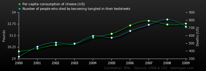
These days, there are so many dubious assertions about alleged correlations between two variables that an entire website: Spurious Correlation (Tyler Vigen) is devoted to exposing (and creating*) them! A classic problem is that the means of variables X and Y may both be trending in the order data are observed, invalidating the assumption that their means are constant. In my initial study with Aris Spanos on misspecification testing, the X and Y means were trending in much the same way I imagine a lot of the examples on this site are––like the one on the number of people who die by becoming tangled in their bedsheets and the per capita consumption of cheese in the U.S.
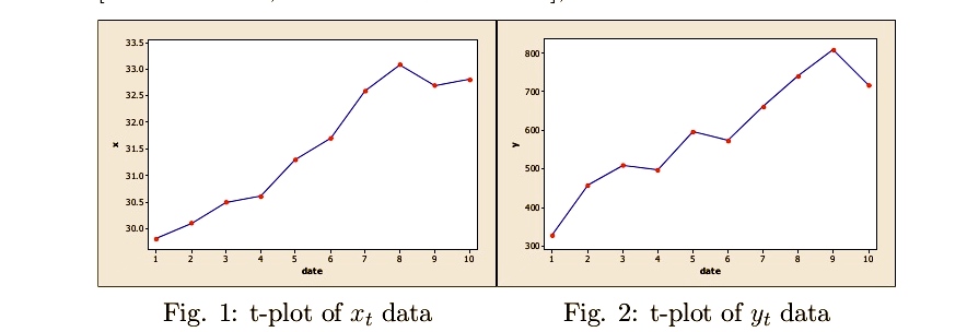
The annual data for 2000-2009 are: xt: per capita consumption of cheese (U.S.) : x = (29.8, 30.1, 30.5, 30.6, 31.3, 31.7, 32.6, 33.1, 32.7, 32.8); yt: Number of people who died by becoming tangled in their bedsheets: y = (327, 456, 509, 497, 596, 573, 661, 741, 809, 717)
I asked Aris Spanos to have a look, and it took him no time to identify the main problem. He was good enough to write up a short note which I’ve pasted as slides.
Aris Spanos
Wilson E. Schmidt Professor of Economics
Department of Economics, Virginia Tech
*The site says that the server attempts to generate a new correlation every 60 seconds.


")


Having done a lot of applied I think both Spanos and the jokey correlation website miss the boat on a couple things here.
Many of the situations being called spurious are not “spurious” at all, but non-random correlations due to a common cause, just not the cause in question (usually a direct effect on one correlate to the other).
The “de-trend the mean” suggestion further muddies the waters. What’s the distinction between the variation that needs to be “de-trended” and one that doesn’t? It’s fundamentally a causal distinction.
There is a well known distinction between high correlation as a result of joint dependence on an omitted variable and what Yule called “nonsense” correlations arising especially from correlating serially correlated variables, where there is no real relation between the variables at all. Granger and Newbold famously showed how two random walks could show high correlation even though, by construction, they were unrelated. I am sure that the latter is a significant potential problem, especially in time series analysis.
vl54321: I have to admit that I did miss one boat. The boat of confusion between statistical and substantive adequacy the permeates your comment. Correlation is primarily a statistical concept, and hence, one needs to establish its statistical meaningfulness first [by validating the probabilistic assumptions that render it meaningful] before embarking on substantive interpretations like a causal claim. A trend provides a generic way one can use to account for heterogeneity in the data in order to establish statistical adequacy. The latter ensures that one’s estimators and tests do have the error-probabilistic properties claimed; consistent estimators, UMP tests, etc. Once that is secured, one can then proceed to consider the substantive question of interest, such as a common cause. The latter can be shown by pinpointing to a substantively meaningful variable z(t) that can replace the trend in the associated regression and also satisfies the correlation connections with y(t) and x(t) required for a common cause. This is the reason I brought out the connection between correlation and linear regression in my note above.
Caution: For those who might consider a trend as a common cause, I urge them to reconsider by consulting informed books on probability and statistics that explain why one cannot condition on a deterministic variable by treating it as a random variable; it is not!
For those who care to avoid the boat of confusion between statistical and substantive adequacy can glance through the following paper:
Spanos, A. (2006), “Revisiting the Omitted Variables Argument: Substantive vs. Statistical Adequacy,” Journal of Economic Methodology, 13: 179–218.
If z(t) = x(t) was deemed ‘substantively meaningful’ in explaining y(t), would you still conclude ‘There is no statistical correlation between these two variables afterall!’.
Furthermore, I assume you would refuse to set up some sort of errors-in-variables or latent variable model and condition on the latent process (e.g. the mean of x(t))?
on the spurious correlation page and almost all applications where investigators search for correlations the data arise from non-randomized, observational data.
In such contexts, “random” variation is only an approximation for missing information regarding the underlying dependency structure. There is no demarcation between so-called systematic and random variation.
The end result is simply that the non-systematic components of y_t and x_t are not related, right? What’s to block the conclusion that the variation in the mean of x_t is driving the changes in the mean of y_t etc?
Or, to quote Cressie’s book Statistics for Spatial Data: “One person’s deterministic mean structure may be another person’s correlated error structure”
omaclaren: anybody who indulges in statistics and cannot distinguish between heterogeneity [e.g. a deterministic trend] and dependence [e.g. correlated error structure] should change hobbies.
Ha.
But anyway, what I see here is – a choice to work in terms of relatively arbitrary ‘de-trended’ variables and an apparent conclusion – that the variables x and y are unrelated because their de-trended versions x* and y* are unrelated – that depends on this choice.
Fine if all of this is supposed to be purely manipulation of a cause-free statistical model in order to put it in some canonical econometric form or whatever, but this then by definition cannot address whether the common linear increasing trend in time is a ‘spurious’ result or not.
Furthermore, I can imagine many simple examples of dynamical systems – e.g. from first year physics – where a common trend is causal and intervening on one variable would affect the other, and many others where it is not and intervening on one would not affect the other. I’m not sure how to address the concept of a ‘spurious’ correlation or relationship – as per the title of the post – without some sort of causal assumption/model or intervention.
I don’t mean this to be too aggressive in tone and I understand this is a relatively quick, simple example, but – what are we actually supposed to take away from this example?
omaclaraen: The example was just to illustrate a “common cause” of spurious correlations, and how it may be unearthed.
It seems to me there are some simple takeaways. Don’t use a deterministic variable like a random variable in a statistical model. Dont neglect a common cause when interpreting correlations. Do control for common cause z if your interest is in the relationship between x and y. To wit, do not interpret a correlation between grade level and body weight as evidence that school makes children fat…
omaclaren: what one is supposed to take from this example is the following: any form of statistical inference, including estimation and testing, depends crucially on the probabilistic assumptions one imposes on the data (implicitly or explicitly); the assumed statistical model. When any of these assumptions are invalid for one’s data, the resulting inferences are spurious (invalid) to a greater or a lesser degree. In the above example, the assumption of a constant mean (a component part of the ID assumption) is invalid for the particular data, and thus the inference result of a highly significant correlation is spurious. This is demonstrated by showing that when the trending mean is accounted for, the resulting inference is totally different; the “apparent” high correlation is a mirage created by invoking false assumptions when estimating and testing the significance of the correlation coefficient.
OK, I take the general point. It’s not that I disagree as such, but that I feel calling a relationship (statistical or not) between two variables spurious or ‘true’ fundamentally involves causality. I’ve had a think and here’s one last amateur attempt to explain the sort of story that I intuitively started to think of when I saw the data. Again, just an alternative perspective, influenced by my background in ‘mechanistic’ modelling (though I’ve taken a fair share of courses in regression in the past, they never really felt natural as compared to e.g. courses in physics or differential equations). I’m sure it’s flawed in many ways, though:
Given two relationships with linear trend in time, y = at, x = bt, obviously one can re-write this as y = (a/b)x. Hence the existence of possible ‘spurious relationships’ between any two trending variables. To me, though, the question of whether this relation between y and x is causal or spurious is related to how these relations vary or not under a range of ‘different’ conditions.
For example, suppose we change some external conditions previously held constant and suppose we already know that this gives a new b, b’ = b/2. If we re-run the regressions and find a also changes as a’=a/2, then the relation y = (a/b)x = (a’/b’)x remains the same. I would say this captures some idea of causality (as opposed to spurious relation or correlation) – ‘a relation or correlation that is invariant under the set of conditions T is causal with respect to T’. Or something.
This would mean e.g. conservation laws (mass, momentum, energy etc) are ‘causal’ under an extremely wide range of conditions, but spurious correlations are only ‘causal’ under a very restricted set of conditions. Causality is then a matter of degree and this can only be determined by examining a range of conditions.
The reason for disbelieving particular relationships is then doubt that they will hold under some ‘intervention’ or change in conditions – they only hold for this particular dataset. Re: John Byrd’s comment: we imagine that we could hold back some kids from advancing in school and watch them still gain weight etc. I note that this is not too dissimilar to the idea of severity – ask how robust a fit is with respect to variations in conditions/parameters.
Anyway, thanks for the responses. It’s been a useful exercise for me to think these things through a bit.