

.
Stephen Senn
Consultant Statistician
Edinburgh
‘The term “point estimation” made Fisher nervous, because he associated it with estimation without regard to accuracy, which he regarded as ridiculous.’ Jimmy Savage [1, p. 453]
First things second
The classic text by David Cox and David Hinkley, Theoretical Statistics (1974), has two extremely interesting features as regards estimation. The first is in the form of an indirect, implicit, message and the second explicit and both teach that point estimation is far from being an obvious goal of statistical inference. The indirect message is that the chapter on point estimation (chapter 8) comes after that on interval estimation (chapter 7). This may puzzle the reader, who may anticipate that the complications of interval estimation would be handled after the apparently simpler point estimation rather than before. However, with the start of chapter 8, the reasoning is made clear. Cox and Hinkley state:
Superficially, point estimation may seem a simpler problem to discuss than that of interval estimation; in fact, however, any replacement of an uncertain quantity is bound to involve either some arbitrary choice or a precise specification of the purpose for which the single quantity is required. Note that in interval-estimation we explicitly recognize that the conclusion is uncertain, whereas in point estimation…no explicit recognition is involved in the final answer. [2, p. 250]
In my opinion, a great deal of confusion about statistics can be traced to the fact that the point estimate is seen as being the be all and end all, the expression of uncertainty being forgotten. For example, much of the criticism of randomisation overlooks the fact that the statistical analysis will deliver a probability statement and, other things being equal, the more unobserved prognostic factors there are, the more uncertain the result will be claimed to be. However, statistical statements are not wrong because they are uncertain, they are wrong if claimed to be more certain (or less certain) than they are.
A standard error
Amongst justifications that Cox and Hinkley give for calculating point estimates is that when supplemented with an appropriately calculated standard error they will, in many cases, provide the means of calculating a confidence interval, or if you prefer being Bayesian, a credible interval. Thus, to provide a point estimate without also providing a standard error is, indeed, an all too standard error. Of course, there is no value in providing a standard error unless it has been calculated appropriately and addressing the matter of appropriate calculation is not necessarily easy. This is a point I shall pick up below but for the moment let us proceed to consider why it is useful to have standard errors.
First, suppose you have a point estimate. At some time in the past you or someone else decided to collect the data that made it possible. Time and money were invested in doing this. It would not have been worth doing this unless there was a state of uncertainty that the collection of data went some way to resolving. Has it been resolved? Are you certain enough? If not, should more data be collected or would that not be worth it? This cannot be addressed without assessing the uncertainty in your estimate and this is what the standard error is for.
Second, you may wish to combine the estimate with other estimates. This has a long history in statistics. It has been more recently (in the last half century) developed under the heading of meta-analysis, which is now a huge field of theoretical study and practical application. However, the subject is much older than that. For example, I have on the shelves of my library at home, a copy of the second (1875) edition of On the Algebraical And Numerical Theory of Observations: And The Combination of Observations, by George Biddell Airy (1801-1892). [3] Chapter III is entitled ‘Principles of Forming the Most Advantageous Combination of Fallible Measures’ and treats the matter in some detail. For example, Airy defines what he calls the theoretical weight (t.w.) for combining errors as![]() and then draws attention to ‘two remarkable results’
and then draws attention to ‘two remarkable results’
First. The combination-weight for each measure ought to be proportional to its theoretical weight.
Second. When the combination-weight for each measure is proportional to its theoretical weight, the theoretical weight of the final result is equal to the sum of the theoretical weights of the several collateral measures. (pp. 55-56).
We are now more used to using the standard error (SE) rather than the probable error (PE) to which Airy refers. However, the PE, which can be defined as the SE multiplied by the upper quartile of the standard Normal distribution, is just a multiple of the SE. Thus we have PE ≈ 0.645 × SE and therefore 50% of values ought to be in the range mean −PE to mean +PE, hence the name. Since the PE is just a multiple of the SE, Airy’s second remarkable result applies in terms of SEs also. Nowadays we might speak of the precision, defined thus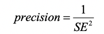
and say that estimates should be combined in proportion to their precision, in which case the precision of the final result will be the sum of the individual precisions.
This second edition of Airy’s book dates from 1875 but, although, I have not got a copy of the first edition, which dates from 1861, I am confident that the history can be pushed at least as far as that. In fact, as has often been noticed, fixed effects meta-analysis is really just a form of least squares, a subject developed at the end of the 18thand beginning of the 19th century by Legendre, Gauss and Laplace, amongst others. [4]
A third reason to be interested in standard errors is that you may wish to carry out a Bayesian analysis. In that case, you should consider what the mean and the ‘standard error’ of your prior distribution are. You can then apply Airy’s two remarkable results as follows.
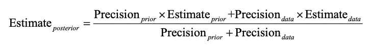
and
![]()
Ignoring uncertainty
Suppose that you regard all this concern with uncertainty as an unnecessary refinement and argue, “Never mind Airy’s precision weighting; when I have more than one estimate, I’ll just use an unweighted average”. This might seem like a reasonable ‘belt and braces’ approach but the figure below illustrates a problem. It supposes the following. You have one estimate and you then obtain a second. You now form an unweighted average of the two. What is the precision of this mean compared to a) the first result alone and b) the second result alone? In the figure, the X axis gives the relative precision of the second result alone to that of the first result alone. The Y axis gives the relative precision of the mean to the first result alone (red curve) or to the second result alone (blue curve).
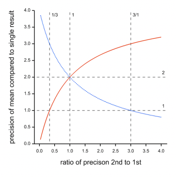
Figure: Precision of an unweighted mean of two estimates as a function of the relative precision of the second compared to the first. The red curve gives the relative precision of the mean to that of the first and the blue curve the relative precision of the mean to the second. If both estimates are equally precise, the ratio is one and the precision of the mean is twice that of either result alone.
Where a curve is below 1, the precision of the mean is below the relevant single result. If the precision of the second result is less than 1/3 of the first, you would be better off using the first result alone. On the other hand, if the second result is more than three times as precise as the first, you would be better off using the second alone. The consequence is, that if you do not know the precision of your results you not only don’t know which one to trust, you don’t even know if an average of them should be preferred.
Not ignoring uncertainty
So, to sum up, if you don’t know how uncertain your evidence is, you can’t use it. Thus, assessing uncertainty is important. However, as I said in the introduction, all too easily, attention focuses on estimating the parameter of interest and not the probability statement. This (perhaps unconscious) obsession with point estimation as the be all and end all causes problems. As a common example of the problem, consider the following statement: ‘all covariates are balanced, therefore they do not need to be in the model’. The point of view expresses the belief that nothing of relevance will change if the covariates are not in the model, so why bother.
It is true that if a linear model applies, the point estimate for a ‘treatment effect’ will not change by including balanced covariates in the model. However, the expression of uncertainty will be quite different. The balanced case is one that does not apply in general. It thus follows that valid expressions of uncertainty have to allow for prognostic factors being imbalanced and this is, indeed, what they do. Misunderstanding of this is an error often made by critics of randomisation. I explain the misunderstanding like this: If we knew that important but unobserved prognostic factors were balanced, the standard analysis of clinical trials would be wrong. Thus, to claim that the analysis of randomised clinical trial relies on prognostic factors being balanced is exactly the opposite of what is true. [5]
As I explain in my blog Indefinite Irrelevance, if the prognostic factors are balanced, not adjusting for them, treats them as if they might be imbalanced: the confidence interval will be too wide given that we know that they are not imbalanced. (See also The Well Adjusted Statistician. [6])
Another way of understanding this is through the following example.
Consider a two-armed placebo-controlled clinical trial of a drug with a binary covariate (let us take the specific example of sex) and suppose that the patients split 50:50 according to the covariate. Now consider these two questions. What allocation of patients by sex within treatment arms will be such that differences in sex do not impact on 1) the estimate of the effect and 2) the estimate of the standard error of the estimate of the effect?
Everybody knows what the answer is to 1): the males and females must be equally distributed with respect to treatment. (Allocation one in the table below.) However, the answer to 2) is less obvious: it is that the two groups within which variances are estimated must be homogenous by treatment and sex. (Allocation two in the table below shows one of the two possibilities.) That means that if we do not put sex in the model, in order to remove sex from affecting the estimate of the variance, we would have to have all the males in one treatment group and all the females in another.
| Allocation one | Allocation two | |||||
| Sex | Sex | |||||
| Male | Female | Male | Female | Total | ||
|
Treatment |
Placebo | 25 | 25 | 50 | 0 | 50 |
| Drug | 25 | 25 | 0 | 50 | 50 | |
| Total | 50 | 50 | 50 | 50 | 100 | |
Table: Percentage allocation by sex and treatment for two possible clinical trials
Of course, nobody uses allocation two but if allocation one is used, then the logical approach is to analyse the data so that the influence of sex is eliminated from the estimate of the variance, and hence the standard error. Savage, referring to Fisher, puts it thus:
He taught what should be obvious but always demands a second thought from me: if an experiment is laid out to diminish the variance of comparisons, as by using matched pairs…the variance eliminated from the comparison shows up in the estimate of this variance (unless care is taken to eliminate it)… [1, p. 450]
The consequence is that one needs to allow for this in the estimation procedure. One needs to ensure not only that the effect is estimated appropriately but that its uncertainty is also assessed appropriately. In our example this means that sex, in addition to treatment, must be in the model.
Here There be Tygers
it doesn’t approve of your philosophy Ray Bradbury, Here There be Tygers
So, estimating uncertainty is a key task of any statistician. Most commonly, it is addressed by calculating a standard error. However, this is not necessarily a simple matter. The school of statistics associated with design and analysis of agricultural experiments founded by RA Fisher, and to which I have referred as the Rothamsted School, addressed this in great detail. Such agricultural experiments could have a complicated block structure, for example, rows and columns of a field, with whole plots defined by their crossing and subplots within the whole plots. Many treatments could be studied simultaneously, with some (for example crop variety) being capable of being varied at the level of the plots but some (for example fertiliser) at the level of the subplots. This meant that variation at different levels affected different treatment factors. John Nelder developed a formal calculus to address such complex problems [7, 8].
In the world of clinical trials in which I have worked, we distinguish between trials in which patients can receive different treatments on different occasions and those in which each patient can independently receive only one treatment and those in which all the patients in the same centre must receive the same treatment. Each such design (cross-over, parallel, cluster) requires a different approach to assessing uncertainty. (See To Infinity and Beyond.) Naively treating all observations as independent can underestimate the standard error, a problem that Hurlbert has referred to as pseudoreplication. [9]
A key point, however, is this: the formal nature of experimentation forces this issue of variation to our attention. In observational studies we may be careless. We tend to assume that once we have chosen and made various adjustments to correct bias in the point estimate, that the ‘errors’ can then be treated as independent. However, only for the simplest of experimental studies would such an assumption be true, so what justifies making it as matter of habit for observational ones?
Recent work on historical controls has underlined the problem [10-12]. Trials that use such controls have features of both experimental and observational studies and so provide an illustrative bridge between the two. It turns out that treating the data as if they came from one observational study would underestimate the variance and hence overestimate the precision of the result. The implication is that analyses of observational studies more generally may be producing inappropriately narrow confidence intervals. [10]
Rigorous uncertainty
If a man will begin with certainties, he shall end in doubts; but if he will be content to begin with doubts he shall end in certainties. Francis Bacon, The Advancement of Learning, Book I, v,8.
In short, I am making an argument for Fisher’s general attitude to inference. Harry Marks has described it thus:
Fisher was a sceptic…But he was an unusually constructive sceptic. Uncertainty and error were, for Fisher, inevitable. But ‘rigorously specified uncertainty’ provided a firm ground for making provisional sense of the world. H Marks [13, p.94]
Point estimates are not enough. It is rarely the case that you have to act immediately based on your best guess. Where you don’t, you have to know how good your guesses are. This requires a principled approach to assessing uncertainty.
References
- Savage, J., On rereading R.A. Fisher. Annals of Statistics, 1976. 4(3): p. 441-500.
- Cox, D.R. and D.V. Hinkley, Theoretical Statistics. 1974, London: Chapman and Hall.
- Airy, G.B., On the Algebraical and Numerical Theory of Errors of Observations and the Combination of Observations. 1875, london: Macmillan.
- Stigler, S.M., The History of Statistics: The Measurement of Uncertainty before 1900. 1986, Cambridge, Massachusets: Belknap Press.
- Senn, S.J., Seven myths of randomisation in clinical trials. Statistics in Medicine, 2013. 32(9): p. 1439-50.
- Senn, S.J., The well-adjusted statistician. Applied Clinical Trials, 2019: p. 2.
- Nelder, J.A., The analysis of randomised experiments with orthogonal block structure I. Block structure and the null analysis of variance. Proceedings of the Royal Society of London. Series A, 1965. 283: p. 147-162.
- Nelder, J.A., The analysis of randomised experiments with orthogonal block structure II. Treatment structure and the general analysis of variance. Proceedings of the Royal Society of London. Series A, 1965. 283: p. 163-178.
- Hurlbert, S.H., Pseudoreplication and the design of ecological field experiments. Ecological monographs, 1984. 54(2): p. 187-211.
- Collignon, O., et al., Clustered allocation as a way of understanding historical controls: Components of variation and regulatory considerations. Stat Methods Med Res, 2019: p. 962280219880213.
- Galwey, N.W., Supplementation of a clinical trial by historical control data: is the prospect of dynamic borrowing an illusion? Statistics in Medicine 2017. 36(6): p. 899-916.
- Schmidli, H., et al., Robust meta‐analytic‐predictive priors in clinical trials with historical control information. Biometrics, 2014. 70(4): p. 1023-1032.
- Marks, H.M., Rigorous uncertainty: why RA Fisher is important. Int J Epidemiol, 2003. 32(6): p. 932-7; discussion 945-8.


")


I’m extremely grateful to Stephen Senn for providing this guest post. We keep hearing about the need to “embrace uncertainty” these days, along with the allegation that frequentist (error) statistics is guilty of the “false promise of certainty.” (e.g., in Wasserstein et al., 2019). It’s quite bizarre, given that every error statistical inference is accompanied by an error probability qualification. These same critics point to Bayesian methods as properly embracing uncertainty, by contrast. Ironically, a posterior probability is not accompanied by an assessment of uncertainty. As David Cox says, “they are what they are”.
I agree that posterior probabilities are what they are, at least in purist versions of the Bayesian approach. In fact, two of my blogs on this website deal explicitly with this. See https://errorstatistics.com/2012/05/01/stephen-senn-a-paradox-of-prior-probabilities/ and https://errorstatistics.com/2013/12/03/stephen-senn-dawids-selection-paradox-guest-post/. However, frequentists must also accept that uncertainty statements themselves are dependent on assumptions and that the assumptions may be wrong.
I seem to recall Efron describing what one would have to do before the Student-Fisher revolution. The uncertainty of the point estimate would depend on the unknown true variance, for which you would plug in a sample variance. If you worried about whether the plug-in variance was reliable, you would estimate the variance of the variance. In theory this could go on for ever. Student found a statistic that did not depend on the unknown variance, provided that one could assume the distribution was Normal.My article in Significance https://rss.onlinelibrary.wiley.com/doi/full/10.1111/j.1740-9713.2008.00280.x illustrates this for a sample of size 2 (Figure 2.) Fisher saw the geometrical representation of what Student had done and set about implementing it more widely.
The bootstrap can be regarded as taking this lack of dependence on assumptions one stage further but the dependence cannot be eliminated completely.
To return to my blog, the main purpose was to stress that making some sort of honest attempt to assess uncertainty is important.
Stephen:
Thank you so much for linking to your Significance paper. I hadn’t known it. So Student studied something other than beer–hours of sleep of inmates in an insane asylum in the U.S.
I was mainly wanting to point up the irony in the latest radical call to “Accept uncertainty”, the A in the ATOM Declaration, along with the refrain I am hearing more and more these days, to wit: that frequentist error statistics claims to give certainties. Maybe I’m just increasingly finding myself in forums with people who have bought into the criticisms embodied in Wasserstein et al 2019: of “the seductive certainty falsely promised by statistical significance.” As I wrote in my “P-value thresholds: Forfeit at your Peril”: “This warning is puzzling, however, given that all error statistical inferences are qualified with error probabilities, unlike many other approaches.”
https://onlinelibrary.wiley.com/doi/epdf/10.1111/eci.13170
Actually I think Cox said, about Bayesian posteriors, that “they are as they are” and are not qualified (not “they are what they are”). I’m guilty for not looking it up. My excuse is that he has also said it to me aloud.
Efron’s point about what one would have to do before the Student-Fisher revolution is very illuminating. (It strikes me that I think this is what I was trying to say on p. 378 of SIST.)
Moving back to your post, is it the epidemiologists you have in mind (who get the wrong estimates of error)? Or the causal modelers?
OK, my first idea for where to find the Cox statement was correct,it’s Cox’s comment on Lindley–a paper that is linked to on my blog (along with the discussion).
“Moreover, so far as I understand it, we are not allowed to attach measures of precision to probabilities. They are as they are. A probability of 1/2 elicited from unspecified and flimsy information is the same as a probability based on a massive high quality database. Those based on very little information are unstable under perturbations of the information set but that is all.”
(p. 323)
Click to access Lindley_Philosophy_of_Statistics.pdf
I’ll stray a little from the discussion that you and Deborah are having to address the concern with uncertainty. Of course, we need to be aware of the uncertainty around both our point predictions and our parameter estimates. And a statement like “statistical statements are not wrong because they are uncertain, they are wrong if claimed to be more certain (or less certain) than they are.” while true doesn’t address an important point – that most people bothered by bad point predictions aren’t bothered because the ‘statistical statements’ are wrong. They are bothered because the models used to make the predictions are wrong.
Missing the target by an enormous amount but being happy because you correctly estimated how much you would miss the target by should be cold comfort to scientists trying to understand how the world works. I suspect there are few scientists who believe the primary objective of science is to estimate precisely how little we know about how the world works. There seems to be a growing philosophy that we should evaluate models based on how well they estimate uncertainty rather than on how close they get to predicting the right answer (and this post seems to reflect that philosophy). When making decisions it is very important to know how much uncertainty there is in a prediction. But, when assessing a model we care about how close the model gets to the right answer – that is, how good the point predictions are.
Jeff Houlahan
Jeff:
First, I don’t know why I wasn’t alerted to your comment.
Second, thanks for your comment. I think the kind of assessment of uncertainty here is intended to be an assessment of how close the estimate is to the right answer. I’ll let Stephen Senn give his thoughts here.
Thanks for your comments, Jeff. In my opinion, however, science is not a static exercise. If we have to make a decision now based on an estimate, then it may be good enough for us to know that the estimate is best in some sense. However, very little of anything I have been involved with in the more than thirty years I have been working in or with drug development is like this. At nearly every stage it is necessary to know how good an estimate is, whether to know how to combine it with other estimates, or whether to know if more time and money needs to be spent collecting further information. Thus, if instead of seeing science as static, you see it as an iteration, it is, indeed, essential to know how well you have estimated what you have estimated.
So, this statement “Missing the target by an enormous amount but being happy because you correctly estimated how much you would miss the target by should be cold comfort to scientists trying to understand how the world works.” does not obviate the need for estimates of uncertainty. Suppose that you have made an estimate. Under what circumstances can you know how the world works? Presumable, to follow your line of argument, if your estimate is sufficiently precise and accurate. But how can you know it is sufficiently precise and if you know why won’t you tell the world? Thus, claiming that what is important is precise and accurate estimation, does not absolve you from the necessity of understanding how good your estimate is. On the contrary, this understanding is crucial to making good estimates and in particular knowing if and how precision increases with ‘sample size’ is central, as I explained in this previous blog.
https://errorstatistics.com/2019/03/09/s-senn-to-infinity-and-beyond-how-big-are-your-data-really-guest-post/
In other words, I deny that in any endeavour in which obtaining information is difficult, you can make good estimates without being able to assess how good they are.
Pingback: S. Senn: Randomisation is not about balance, nor about homogeneity but about randomness (Guest Post) | Error Statistics Philosophy