

.
Stephen Senn
Head of Competence Center for Methodology and Statistics (CCMS)
Luxembourg Institute of Health
Twitter @stephensenn
Painful dichotomies
The tweet read “Featured review: Only 10% people with tension-type headaches get a benefit from paracetamol” and immediately I thought, ‘how would they know?’ and almost as quickly decided, ‘of course they don’t know, they just think they know’. Sure enough, on following up the link to the Cochrane Review in the tweet it turned out that, yet again, the deadly mix of dichotomies and numbers needed to treat had infected the brains of researchers to the extent that they imagined that they had identified personal response. (See Responder Despondency for a previous post on this subject.)
The bare facts they established are the following:
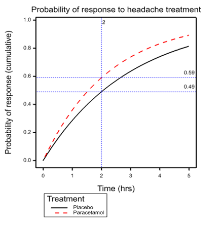
The International Headache Society recommends the outcome of being pain free two hours after taking a medicine. The outcome of being pain free or having only mild pain at two hours was reported by 59 in 100 people taking paracetamol 1000 mg, and in 49 out of 100 people taking placebo.
and the false conclusion they immediately asserted is the following
This means that only 10 in 100 or 10% of people benefited because of paracetamol 1000 mg.
To understand the fallacy, look at the accompanying graph. This shows the simplest possible model describing events over time that is consistent with the ‘facts’. The model in question is the exponential distribution and what is shown is the cumulative probability of response for individuals suffering from tension headache depending on whether they are treated with placebo or paracetamol. The dashed vertical line is at the arbitrary International Headache Society critical time point of 2 hours. This intersects the placebo curve at 0.49 and the paracetamol curve at 0.59, exactly the figures quoted in the Cochrane review.
 The model that the diagram represents is simplistic and almost certainly false. It is what would apply if it were the case that all patients given placebo had the same probability over time of headache resolution and ditto for paracetamol and an exponential model applied. However, the point is that for all we know it is true. It would take careful measurement over time for repeated headaches of the same individuals to establish the element of personal response (Senn 2016).
The curve given for placebo is what we would expect to find for the simple exponential model if it were the case that mean time to response were 2.97 hours when a patient was given placebo. The curve for paracetamol has a mean of 2.24 hours. It is important to understand that this is perfectly compatible with this being the long term average response time (that is to say averaged over many many headaches) for every patient and this means that any patient at any time feeling the symptoms of headache could expect to shorten that headache by 2.97-2.24=0.73 hrs or just under 45 minutes.
Is this a benefit or not? I would say, ‘yes’. And that means that a perfectly logical way to describe the results is to say, ‘for all we know, any patient taking paracetamol for headache will benefit. The size of that benefit is an increase of the probability of resolution at 2 hours of 10 percent or a reduction of mean headache time of 3/4 of an hour’.
The latter, of course, depends on the exponential model being appropriate and it may be that some alternative can be found by careful analysis of the data. The point is, however, that the claim that only 10% will benefit by taking paracetamol is completely unjustified.
Unfortunately, the combination of arbitrary dichotomies (Senn 2003) and naïve analysis continues to fuel misunderstandings regarding personalised medicine.
Acknowledgement:
This work was funded by grant 602552 for the IDEAL project under the European Union FP7 programme and support from the programme is gratefully acknowledged.
References:
- S. J. Senn (2003) Disappointing dichotomies. Pharm Stat, 239-240.
- S. J. Senn (2016) Mastering variation: variance components and personalised medicine. Stat Med, 966-977.


")


When I said “The size of that benefit is an increase of the probability of resolution at 2 hours of 0.1 percent…” I meant, of course, The size of that benefit is an increase of the probability of resolution at 2 hours of 10 percent” but then what’s a factor of 100 here or there?
I’ll change it.
Thanks. I appreciate it.
Great post. The problem seems a more basic and general version of that pointed out by Robins and I many years ago, that any increase in average risk or response seen in one group over another may stem from a small improvement in everyone or a much larger improvement in a few, so that standard measures of attributable risk or benefit are not (as commonly misinterpreted) measures of the proportion harmed or benefitted, or the ‘probability of causation’ (e.g., Greenland Robins, Am J Epidemiol 1988,128:1185-97; Robins Greenland Biometrics 1989, 46:1125-38). Unfortunately the latter misinterpretation seems so widespread and compelling that we have had to write expository articles about it ever since (e.g., Greenland, Am J Public Health 1999, 89:1166-9; Beyea Greenland 1999; Health Physics 76:269-74) yet it persists.
Ed note: Link I had: https://errorstatistics.files.wordpress.com/2016/08/greenland-robins-1988.pdf
Thanks Sander for the comments and also for the references, which I shall study. Another important paper that you could have cited is Rothman KJ, Greenland S, Walker AM. Concepts of interaction. American Journal of Epidemiology 1980; 112:467–470.
Recently, I cited this as follows:
“A key paper is that of Rothman, Greenland and Walker [44] who draw a careful distinction between statistical and biologic interaction ”
http://onlinelibrary.wiley.com/doi/10.1002/sim.6739/abstract
Thanks Stephen…The effects Robins & Greenland 1989 consider involve one more complication besides interaction: noncollapsibility. It is possible for there to be no interaction at all and yet have the usual causal or preventive attribution measures be much less than the actual proportion of responses caused by treatment.
The event-time effects you consider (which we wrote about in Robins Greenland Stat Med 1991; 10:79-93) are more general in that they need not involve noncollapsibility; and their misinterpretations may be viewed as a simple failure to realize that a mean response is just that and no more, leaving open possibilities of anything from zero to universal interaction. For example if we observe identical survival curves in both groups that may represent anything from no effect on anyone (the Fisher null, and I think the usual interpretation) to the implausible opposite extreme of 50% who benefit from treatment, and 50% who are harmed by it and respond in exactly the opposite way. The latter case satisfies the Neyman null (no average causal effect), which Gelman defends but I see as encouraging interaction blindness: In the presence of qualitative interactions involving unmeasured covariates, statistical data cannot distinguish among rather extreme alternatives and the Fisher (sharp) null. This does not mean we should pretend that all the hypotheses lumped into the Neyman null are operationally equivalent, or forego trying to identify possible qualitative interactions. (I was fortunate in being alerted to this problem early on: The data I used in my dissertation exhibited zero average effect, which turned out to be an average of 3/4 of the patients exhibiting moderate harms and 1/4 exhibiting great benefits – as predicted by some clinicians wary of applying the treatment to all patients.)
I think underlying these continual misunderstanding there is a “statistical world view” that is simply inadequate to fully grasp the issue clearly enough to get it and commit to acting on it (maybe their views can be unfrozen and changed but not quite refrozen so they revert or become paralyzed as not fully sure).
My experience comes with working with many statisticians involved in Cochrane Methods and reviews primarily trying to get across concepts of likelihood and likelihood based statistics (ala David Cox) between 2001 and 2010.
I think I had so little impact that if anything, if since 2010 any have learned about likelihood based statistics they won’t connect that to anything I did with them (Stephen will understand this more than others).
A particular instance was with my office mate who after I went through a tutorial on likelihood based statistics, step by step on our office white board said – “I can not see anything wrong with what you just said – but I just can not accept that it is true!”
Some of that material was published here http://www.ncbi.nlm.nih.gov/pubmed/16118810 though I don’t think that publication indicated any success in actually getting the ideas across to anyone.
I am not trying to be disparaging here, I really think there is something they missed in their statistical education that makes thinking in terms of models and parameters instead of techniques, estimators and distributions very difficult.
Keith O’Rourke
Phanero: Can you explain a bit, in relation to the problem Stephen discusses, what you mean in saying: “I really think there is something they missed in their statistical education that makes thinking in terms of models and parameters instead of techniques, estimators and distributions very difficult.”
I’m not sure that i’m getting this so I would like some help. I should add that the concept of personalized medicine is new to me.
If we strip away all the detail from the post then we are being asked to compare two statements, the first of which is wrong but the second is correct:
1 This means that only 10 in 100 or 10% of people benefited (at two hours – my insertion).
2 The size of that benefit is an increase of the probability of resolution at 2 hours of 10%.
The difference between these two statements is going to be too subtle for a lot of people without extra qualification. Is the (non stated) problem with statement 1 that it will be the same 10% of people every time.
Yes, that’s part of the problem but there are others. If you look at the curves on my diagram I could get the paracetamol one by simply shrinking every point on the placebo curve in the X dimension by 1/4 so for all I know that’s what happened. Every single patient on every single occasion had his or her headache duration reduced to 3/4 of what it would have been under placebo. (In fact I have a simulation that demonstrates this and if I could find some way of adding the graph here would.)
Now you could argue, “in some cases that was quite a lot of reduction, but not always. For the average placebo headache it was 45 minutes but for some shorter headaches rather less and then again for some others rather more.”
However, suppose that you are a patient that has to decide whether to take paracetamol or not. If you know nothing about yourself that differentiates you just have to play the averages. That’s it. You can expect that on average you will get a headache that is 45 minutes shorter.
Of course given more information in particular repeat modelling of time courses (some sort of frailty model) you could do better and provide patients with information that might, given some personal headache history, help them come to a better decision. You could maybe start to distinguish patients who benefit and those who don’t.
However, to say that only 10% of patients benefitted is completely unjustified. For all that the figures they quote say, 100% did.
See also my previous post https://errorstatistics.com/2014/07/26/s-senn-responder-despondency-myths-of-personalized-medicine-guest-post/ and in particular the third figure.
What makes me so angry about this is that somewhere, somebody will assume that this sort of meta-analysis justifies looking for a gene for paracetamol response. It doesn’t.
Numbers needed to treat are the work of the devil. Cochrane really needs to get its house in order.
Thanks, Keith. From the abstract your publication with Doug Altman look extremely interesting. However, it is not immediately obvious to me that it refers to assessing individual response. Have you linked to the right text?
I was obviously too vague in what I was trying to get across.
In your example, folks directly observe the two proportions at 2 hours and they can calculate the difference. If they are being overly empirical and not willing to go anywhere beyond the data (what I suspect) they will be wary of your probability generating model that gives an explanation of how those observed proportion could have come about and what one should then make of such observations. Seems a bit too theoretical whereas they know what they have observed and trust the simple arithmetic they brought to bear upon it.
I thought this aspect was similar to my experience in trying to get across likelihood in meta-analysis to a group of well seasoned meta-analytic statisticians that were used to taking observed summary statistics and applying simple arithmetic to to these (inverse variance weighted combinations). The story (representation) of how the summary statistics could have been generated by a probability generating model seemed to be too much for them too entertain – too theoretical, too far removed from the data.
Speculating why others do not understand what one is trying to get across is very speculative – but over a period of seven years, dozens of face to face meetings and hundreds of hours of exchanging papers and emails – there has to be something that is not translating.
Keith O’Rourke
Phanerono:
“The story (representation) of how the summary statistics could have been generated by a probability generating model seemed to be too much for them too entertain – too theoretical, too far removed from the data.”
I’m guessing, in that case, that a prior distribution would be even more abstract?
One would think so, but with WinBugs that had default priors largely hidden in background, Bayesian meta-analysis seemed like a set of alternative procedures that could be applied to the study estimates and standard errors (taken as known). More complicated arithmetic but that did not need to be understood as WinBugs did it.
Its having the think carefully about the various possible representations of an underlying reality that’s being enabled by data generating models (and priors if used) and the abstractness/fallibility of that, that I think folks find too hard.
Taking the study estimates and standard errors (standard error again taken as known rather than just an estimate) and working with them as something usually approximately Normally distributed is so much more concrete and comforting. Any concerns can then be simply addressed by simulation studies of performance – no need to think abstractly.
One more reading related to this http://onlinelibrary.wiley.com/doi/10.1002/sim.2639/abstract
Keith O’Rourke
“WinBugs that had default priors largely hidden in background,”
In WinBugs any analysis has to specify the prior; without it the model won’t compile and no output is produced. So while it’s a challenge to think about what the prior says about underlying reality, the prior is not “hidden” and not “background”. Perhaps you meant some other software?
I agree with Stephen. This is similar to the annoying level of information drug reps have been using for years to try to persuade doctors to prescribe. In this case, the same approach is being used to dissuade doctors from prescribing. I would be interested to know how he thinks the ‘take away message’ should have been phrased. Also could he summarize the best way of conducting a study to provide sensible evidence for the ‘take away message’ that “This means that only 10 in 100 or 10% of people benefited because of paracetamol 1000 mg”?
I have to say that my idea of personalized medicine is for doctors, nurses, etc to adjust what is done to the patient to get the best possible outcome. This is a process of feedback control, which is how the body itself corrects disturbance, e.g. regulating sugar levels, blood pressure, integrity of the skin after injury etc. The doctor’s job is to supplement and not to interfere with these mechanisms. So, to my mind ‘personalized’ medicine can only be performed by the person helping the patient (doctor, nurse etc).
‘Personalized’ medicine must not be confused with ‘accurate’ medicine which is getting predictions right about what will happen with and without interventions of various kinds to a high degree of accuracy, which is often referred to as ‘personalized’ medicine. The only way to do this perfectly for each person is with the aid of a wizard’s crystal ball (which is what some excited people seem to think that they are about to invent).
The traditional way is to select patients for treatment so that as many as possible respond to a specified treatment and in a way that few people respond to placebo. This often depends on the severity or duration of the illness – the very mild or of recent onset often get better anyway (e.g. on placebo) and the very severe fail to get better on treatment (or placebo of course). It is often the case of finding those in the middle ground who ‘benefit’. The degree of benefit often depends on the degree of severity or duration or some other predictive finding. (This is called ‘triage’ in emergency situations.) The answer lies in improving the accuracy of diagnosis – improving the way we match a patient’s illness to a specified treatment (the new word for this is ‘stratification’) and then helping the patient to choose. This requires a far more sophisticated approach to randomized clinical trials.
As far as I can see, neither the EBM establishment nor the Pharmaceutical Industry have understood this yet and are simply demonstrating (as illustrated by Stephen) that a little bit of knowledge is a dangerous thing.
Thanks, Huw. As regards a suitable design, then the key to identifying individual response is replication. Replication has to take place at the level that an interaction is claimed. Thus, if you wish to claim individual patient effects a good design would be to carry out a suite of n-of-1 designs. For example, each of several patients could be treated in each of two cycles whereby each cycle would involve two subsequent headaches, one treated with placebo and one with paracetamol, the order being randomised. This would then permit a model to be fitted that could separate pure differences between patients (some suffer worse than others), differences within patients (even for the same patient given the same treatment not every headache is the same) and treatment by patient interaction (for some paracetamol works betters than others.).
I have advocated this design on several occasions. See, for example the Mastering Variation paper I referred to previously http://onlinelibrary.wiley.com/doi/10.1002/sim.6739/abstract and also a short piece in the BMJ some years ago http://www.bmj.com/content/329/7472/966 . It is also the third of three things I considered that every medical writer should know about statistics in this paper http://eprints.gla.ac.uk/8107/1/id8107.pdf
Your stratification suggestion, of course, is a valid one: interaction can then be assessed at the stratum level but not at the sub-stratum one.
As regards your example of the moderately ill responding best, this might correspond to the effect being (approximately) constant on a scale other than the risk difference scale (for example, the log-odds scale). Translation onto a relevant benefit scale may then be possible. Elsewhere in science this happens all the time. For example, net vehicle velocity is a relevant scale for accident survivability but Newton’s laws involve acceleration. However, any physicist or engineer can translate from one to the other.
Huw posed the question:
“could he summarize the best way of conducting a study to provide sensible evidence for the ‘take away message’ that “This means that only 10 in 100 or 10% of people benefited”
Stephen began his reply by saying:
As regards a suitable design, then the key to identifying individual response is ………….
But Huw’s question didn’t mention individual response and it is not clear to me why Stephen assumed it did.
But if 10% benefitted and 90% did not that is individual response and I provided the way to study it. Without repeated measurements you simply can’t make this sort of statement, so you shouldn’t.
Otherwise one should just shut up
“Whereof one cannot speak, thereof one must be silent.”
Stephen:
First, thanks so much for the guest post.
I took your point to be that it may be that everyone gets a benefit in reduction of time to headache relief, but that by dichotomizing at a given time (decent relief at time t), they report on proportions with and without the characteristic: relief at time t. Whereas, had they chosen to make an inference about mean reduction in time to relief, or something like that, they might have reported everyone gets some benefit. I mean, why look at “relief in 2 hours”? Is that your point?
Wouldn’t you also complain about an inference to the % in the population in general (based on the dichotomized result)?
Yes the dichotomisation is part of the problem but it’s not just that. Suppose that we had some perfect headache guinea-pigs who can be relied on to have a tension headache for at least 5 hours when they get one and it’s not treated. We now take a 1000 and treat them the next time they have a headache and suppose, unrealistically they divide into two sharp classes: 700 have their headache disappear in under two hours whereas for 300 it lasts at least 5.
All the world now takes this to mean that we have shown that the treatment works for 70% of sufferers 100% of the time. But the result would be just the same if it worked for 100% of sufferers 70% of the time. Of course many intermediate positions are possible. How do we tell what’s right? Treating them more than once is a start!
The issue is discussed in more detail in my freely available paper Mastering Variation
http://onlinelibrary.wiley.com/doi/10.1002/sim.6739/abstract
Stephen: I see now, together with your other comment, what this has to do with personalized medicine. I will read your paper, thanks for giving us the link.
Aren’t you also bothered by their reporting the proportions observed as grounding a claim about the general population without some report of precision or statistical significance?
Yes, treating them more than once would be revealing.
Each person may have their own distribution of headache duration. I know I do!
In the report, of course, they use inferential statistics such as confidence intervals. This is standard for Cochrane Collaboration meta-analysis and, indeed, generally, although very few, in doing this, make a distinction between randomisation (which takes place in clinical trials) and random sampling (which does not). In that connection Ludbrook and Dudley (1998) is an interesting paper https://www.jstor.org/stable/2685470?seq=1#page_scan_tab_contents
More generally one cannot simply generalise from clinical trials to general practice although finding additive scales may help. See Added Values http://onlinelibrary.wiley.com/doi/10.1002/sim.2074/abstract
In ecotoxicology we regularly fit probit models to data in which the doses span the range from sub lethal to lethal. The purpose of the exercise is to estimate an LD50, which is required by and duly passed on to regulators. Until recently I was unaware of anyone worrying too much about the mechanisms that result in death or survival, but recently Ashuaer (2013) (and possibly others before him) have been using two distinct models: the IT model (individual tolerance) in which the same animals would die under a hypothetical repeat dosing of the same sample of animals at a given dose; and the SD model (not sure what SD stands for) in which a different 50% of the sample would die under a hypothetical repeat dosing at the LD50.
I’m guessing that the IT model corresponds to your 70% of sufferers 100 of the time, and the SD model corresponds to your 100% of sufferers 70 % of the time.
The difference between IT and SD in ecotoxicology is currently not very important, although that may change. However it must be very important in pharms. If I had a new drug that was never going to be effective in 30% of the population but be very effective on the 70% I would want to know that and I would want to know what it was about 30% that made them different to the 70%. I would therefore design and run tests to explore the issue.
Is this not what happens in pharms???
Ashuer et. al. Environmental Toxicology and Chemistry, Vol. 32, No. 4, pp. 954–965, 2013
Thanks for the reference. (The first author needs to be corrected to Ashauer). This is extremely interesting.I note that one of the addresses they write from is Syngenta, a successor company to CIBA-Geigy, which is one I worked for 1987-1995 (albeit in a different division). They had a statistics group that was active in toxicology amongst other matters and used Bayesian methods as long ago as the early 1980s.
Yes the IT and SD models correspond to the two extremes I gave. I have no idea what SD could stand for unless it is Sprague-Dawley as a sort of paradigm of genetic uniformity which might, in turn, imply that the only source of variation left is environmental, the genetic component being zero.
We have colleagues here at the Luxembourg institute of Health who do work on measuring uptake of pollutants in hair samples (rat and human) and they consult the Competence Center from time to time, so it is useful to me to have a reference to developments in toxicology, especially one that mirrors my own clinical trial work. Thanks.
IT is for individual tolerance and SD for stochastic death.
Perhaps more fully explained in A Unified Probabilistic Framework for Dose-Response Assessment of Human Health Effects. http://www.ncbi.nlm.nih.gov/pmc/articles/PMC4671238/
or more concisely on page 1404 of Exploring the uncertainties in cancer risk assessment using the integrated probabilistic risk assessment (IPRA) approach. http://onlinelibrary.wiley.com/doi/10.1111/risa.12194/abstract
Keith O’Rourke
It might be helpful to think of a situation of the researchers only recording or making available the numbers with/without “relief in 2 hours” in the two groups and nothing more.
Stephen’s model is still as reasonable for how that data may have arise, but there is less information to inform it.
On the other hand, all the information is available for a binomial model of constant independent probability of “relief in 2 hours” in the two separate groups. That does not make it a better model, just a model for which you have all the sample information assuming that model is exactly true (easily false if the probability varies within the groups).
Now with likelihood, one can access all of the information available for Stephen’s model that is in the reported data. (That was my DPhil thesis with a lot of kind input from David Cox.)
Its comes directly from the definition of the likelihood as the probability of what was reported (numbers with/without “relief in 2 hours”) for each and every possible parameter value in Stephen’s model. Unfortunately that used to be very hard to calculated – but today it is trivial using two stage rejection sampling or ABC.
But you have to explicitly write down a probability model for data generation that you know won’t be exactly correct and you are never quite sure if you should repeat the process for some other reasonable models. Not standard practice you can nicely set out in a handbook.
Keith O’Rourke