

.
Stephen Senn
Consultant Statistician
Edinburgh
The intellectual illness of clinical drug evaluation that I have discussed here can be cured, and it will be cured when we restore intellectual primacy to the questions we ask, not the methods by which we answer them. Lewis Sheiner1
Cause for concern
In their recent essay Causal Evidence and Dispositions in Medicine and Public Health2, Elena Rocca and Rani Lill Anjum challenge, ‘the epistemic primacy of randomised controlled trials (RCTs) for establishing causality in medicine and public health’. That an otherwise stimulating essay by two philosophers, experts on causality, which makes many excellent points on the nature of evidence, repeats a common misunderstanding about randomised clinical trials, is grounds enough for me to address this topic again. Before, however, explaining why I disagree with Rocca and Anjum on RCTs, I want to make clear that I agree with much of what they say. I loathe these pyramids of evidence, beloved by some members of the evidence-based movement, which have RCTs at the apex or possibly occupying a second place just underneath meta-analyses of RCTs. In fact, although I am a great fan of RCTs and (usually) of intention to treat analysis, I am convinced that RCTs alone are not enough. My thinking on this was profoundly affected by Lewis Sheiner’s essay of nearly thirty years ago (from which the quote at the beginning of this blog is taken). Lewis was interested in many aspects of investigating the effects of drugs and would, I am sure, have approved of Rocca and Anjum’s insistence that there are many layers of understanding how and why things work, and that means of investigating them may have to range from basic laboratory experiments to patient narratives via RCTs. Rocca and Anjum’s essay provides a good discussion of the various ‘causal tasks’ that need to be addressed and backs this up with some excellent examples.
It’s not about balance and it’s not about homogeneity
In discussing RCTs Rocca and Anjum write
‘…any difference in outcome between the test group and the control group should be caused by the tested interventions, since all other differences should be homogenously distributed between the two groups,’
and later,
‘The experimental design is intended to minimise complexity—for instance, through strict inclusion and exclusion criteria’.
However, it is not the case that randomisation will guarantee that any difference between the groups should be caused by the intervention. On the contrary, many things apart from the treatment will affect the observed difference. And it is not the case that the analysis of RCTs requires the minimisation of complexity. Randomisation and its associated analysis deals with complexity in the experimental material and although the treatment structure in RCTs is often simple this is not always so (I give an example below) and it was not so in the field (literally) of agriculture for which Fisher developed his theory of randomisation. This is what Fisher, himself had to say about complexity
No aphorism is more frequently repeated in connection with field trials, than that we must ask Nature few questions, or ideally one question, at a time. The writer is convinced that this view is wholly mistaken. Nature, he suggests, will best respond to a logical and carefully thought out questionnaire; indeed, if we ask her a single question, she will often refuse to answer until some other topic has been discussed.3 (p. 511)
This 1926 paper of Fisher’s is an important and early statement of his views on randomisation and was cited recently by Simon Raper in his article in Significance4. Raper points out, that Fisher was abandoning as unworkable an earlier view of causality due to John Stuart Mill whereby controlling for everything imaginable was the way you made valid causal judgements. I consider Raper is right in thinking of Fisher’s approach as an alternative to Mill’s programme, rather than some realisation of it, so I disagree for example, with Mumford and Anjum in their book5 when they state
‘Fisher’s idea is the basis of the randomized controlled trial (RCT), which builds on J.S. Mill’s earlier method of difference’ (pp. 111-112).
I shall now explain exactly what it is that Fisher’s approach does with the help of an example.
Breathing lesson
Before going into the example, which is a complex design, it is necessary to clear up one further potential point of confusion in Rocca and Anjum’s essay. N-of-1 studies, are not alternatives to RCTs but a subset of them. RCTs include not just conventional parallel group trials but also cluster randomised trial and cross-over trials, including n-of-1 studies. The difference between these studies is at the level one randomises and this is reflected in my example, which has features of both a parallel group and a cross-over study. Thus, reading Rocca and Anjum’s paper, which I can recommend, will make more sense if by their use of RCT is understood ‘randomised parallel group trials’.
For the moment, all that it is necessary to know is that within the same design, I can compare the effect on forced expiratory volume in one second (FEV1), measured 12 hours after treatment, of two bronchodilators in asthma, which here I shall just label ISF24 and MTA6, in two different ways. First, I can use 71 patients who were given MTA6 and ISF24 on different occasions. Here I can compare the two treatments patient by patient. These data have the structure of a within-patient study. Second, within the same study there were 37 further patients who were given MTA6 but not 1SF24 and 37 further patients who were given ISF24 but not MTA6. Here I can compare the two groups of patients with each other. These data have the structure of a between-patient or parallel group study.
I now proceed to analyse the data from the 71 pairs of values from the patients who were given both using a matched pairs t-test. This will be referred to as the within-patient study. Note that this is an analysis of 2×71=142 values in total. I then proceed to compare the 37 patients given MTA6 only to the 37 given ISF24 only using a two-sample t-test. I shall refer to this as the between-patient study. Note that this is an analysis of 37+37=74 values in total. Finally, I combine the two using a meta-analysis.
The results are presented in the figure below which gives the point estimates for the difference between the two treatments and the 95% confidence intervals for both analyses and for a meta-analysis of both, which is labelled ‘combined’. (The horizontal dashed line is the point estimate for a full analysis of all the data and is described in the appendix.) Note how much wider the confidence intervals are for the between-patient study than the within-patient study. This is because the within-patient study is much more precise.
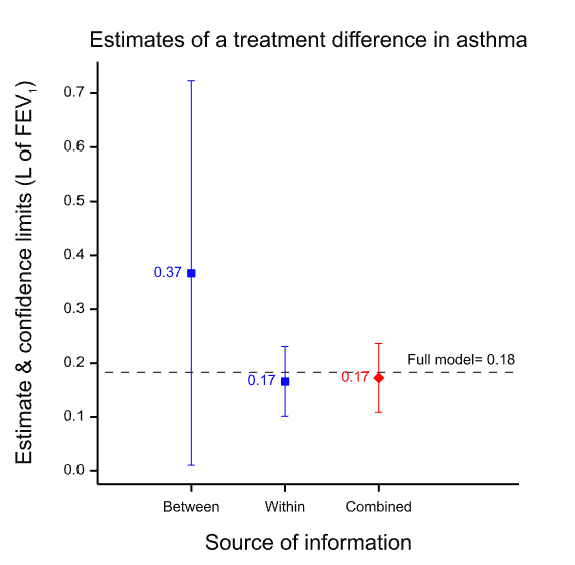
Figure 1 Point estimates and confidence intervals for the between, within and combined estimates.
Why is the within-patient study so much more precise? Part of the story is that it is based on more data, in fact nearly twice as many data: 142 rather than 74. However, this is only part of the story. The ratio of variances is more than 30 to 1 and not just approximately 2 to 1, as the number of data might suggest. The main reason is that the within-patient study has balanced for a huge number of factors and the between-patient study has not. Thus, differences in 20,000 plus genes and all life-history until the beginning of the trial are balanced in the within-patient study, since each patient is his or her own control. For the between-patient study none of this is balanced by design. In fact, there are two crucial points regarding balance.
1. Randomisation does not produce balance
2. This does not affect the validity of the analysis
Why do I claim this does not matter? Suppose we accept the within-patient estimate as being nearly perfect because it balances for those huge numbers of factors. It seems that we can then claim that the between-patient estimate did a pretty bad job. The point estimate is 0.2L more than that from the within-patient design, a non-negligible difference. However, this is to misunderstand what the between-patient analysis claims. Its ‘claim’ is not the point estimate; its claim is the distribution associated with it, of which the 95% confidence interval is a sort of minimalist conventional summary and of which the point estimate is only one point. As I have explained elsewhere, such claims of uncertainty are a central feature of statistics. Thus, the true claim made by the between-patient study is not misleading. It is vague and, indeed, when we come to combine the results, the meta-analysis will give 30 times the weight to the within-patient estimate as to the between-patient estimate simply because of the vagueness of the associated claim. This is why the result from the meta-analysis is so similar to that of the within-patient estimate. Furthermore, although this can never be guaranteed, since probabilities are involved, the 95% CI for the between-patient study includes the estimate given by the within-patient study. (Note, that in general, confidence intervals are not a statement about a value in a future study, but about the ‘true’ average value6 but here, the within-patient study being very precise, they can be taken to be similar.)
How this works
This works because what Fisher’s analysis does is use variation at an appropriate level to estimate variation in the treatment estimate. So, for the between-study it starts from the following observations
1) There are numerous factors apart from treatment that could affect the outcome in one arm of the between-patient study compared to the other.
2) However, it is the joint effect of these that matters.
3) This joint effect of such factors will also vary within each of the two treatment groups.
4) Provided I use a method of allocation that is random, there will be no tendency for this variation within the groups to be larger or smaller than that between the groups.
5) Under this condition I have a way of estimating how reliable the treatment estimate is.
Thus, his programme is not about eliminating all sources of variation. He knows that this is impossible and accepts that estimates will be imperfect. Instead, he answers the question: ‘given that estimates are (inevitably) less than perfect, can we estimate how reliable they are?’. The answer he provides is ‘yes’ if we randomise.
If we now turn to the within-patient estimate, the same argument is repeated but in a first step differences are calculated by patient. These differences do not reflect differences in genes etc. since each patient acts as his or her own control. (They could reflect a treatment-by-patient interaction but this is another story I choose not to go into here7, 8. See my blog on n-of-1 trials for a discussion.) The argument then uses the variance in the single group of differences to estimate how reliable their average will be.
Note that a different design requires a different analysis and in particular because the estimate of the variability of the estimate will be inappropriate even if the estimate is not affected. This is illustrated in Figure 2 which shows what happens if you analyse the paired data from the 71 patients as if they were two independent sets of 71 each. Although the point estimate is unchanged, the confidence interval is now much wider than it was before. The value of having the patients as their own control is lost. The downstream effect of this is that the meta-analysis now weights the two estimates inappropriately.
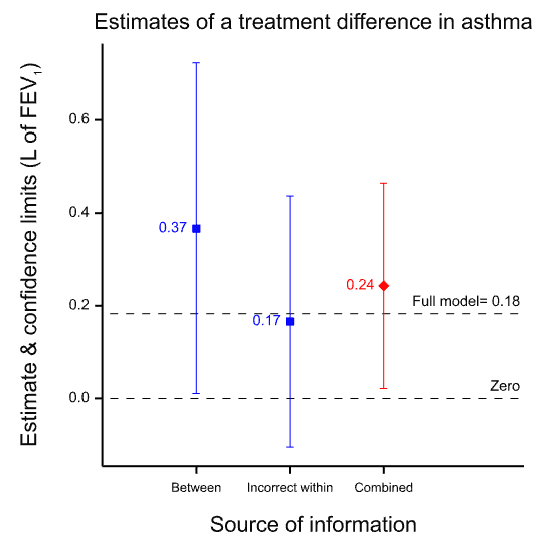
Figure 2 Effect of analysing the within-patient information incorrectly as if it were between-patient. The point estimate is unchanged but the confidence limits are too wide and this in turn leads to the between-patient estimate being given too much weight in the meta-analysis.
Note also, that it is not a feature of Fisher’s approach that claims made by larger or otherwise more precise trials are generally more reliable than smaller or otherwise less precise ones. The increase in precision is consumed by the calculation of the confidence interval9, 10. More precise designs produce narrower intervals. Nothing is left to make the claim that is made more valid. It is simply more precise. The allowance for chance effects will be less, and appropriately so. Balance is a matter of precision not validity.
The shocking truth
As I often put it, the shocking truth about RCTs is the opposite of what many believe. Far from requiring us to know that all possible causal factors affecting the outcome are balanced in order for the conventional analysis of RCTs to be valid, if we knew all such factors were balanced, the conventional analysis would be invalid. RCTs neither guarantee nor require balance. Imbalance is inevitable and Fisher’s analysis allows for this. The allowance that is made for imbalance is appropriate provided that we have randomised. Thus, randomisation is a device for enabling us to make precise estimates of an inevitable imprecision.
Acknowledgements
I thank George Davey Smith, Elena Rocca and Rani Lill Anjum for helpful comments on an earlier version.
References
- Sheiner LB. The intellectual health of clinical drug evaluation [see comments]. Clin Pharmacol Ther 1991; 50(1): 4-9.
- Rocca E, Anjum RL. Causal Evidence and Dispositions in Medicine and Public Health. International Journal of Environmental Research and Public Health 2020; 17.
- Fisher RA. The arrangement of field experiments. Journal of the Ministry of Agriculture of Great Britain 1926; 33: 503-13.
- Raper S. Turning points: Fisher’s random idea. Significance 2019; 16(1): 20-23.
- Mumford S, Anjum RL. Causation: a very short introduction: OUP Oxford, 2013.
- Senn SJ. A comment on replication, p-values and evidence S.N.Goodman, Statistics in Medicine 1992; 11: 875-879. Statistics in Medicine 2002; 21(16): 2437-44.
- Senn SJ. Mastering variation: variance components and personalised medicine. Statistics in Medicine 2016; 35(7): 966-77.
- Araujo A, Julious S, Senn S. Understanding Variation in Sets of N-of-1 Trials. PloS one 2016; 11(12): e0167167.
- Senn SJ. Seven myths of randomisation in clinical trials. Statistics in Medicine 2013; 32(9): 1439-50.
- Cumberland WG, Royall RM. Does Simple Random Sampling Provide Adequate Balance. J R Stat Soc Ser B-Methodol 1988; 50(1): 118-24.
- Senn SJ, Lillienthal J, Patalano F, et al. An incomplete blocks cross-over in asthma: a case study in collaboration. In: Vollmar J, Hothorn LA, eds. Cross-over Clinical Trials. Stuttgart: Fischer, 1997: 3-26.
Appendix: The design of MTA/02
This was a so-called balanced incomplete blocks design necessitated because it was desired to study seven treatments (three doses of each of two formulations and a placebo)11 but it was not considered practical to treat patients in more than five treatments. Thus, patients were allocated a different one of the seven treatments in each of the five periods. That is to say, each patient received a subset of five of the seven treatments. Twenty-one sequences of five treatments were used. Each sequence permits (5×4)/2 = 10 pairwise comparisons but there are (7×6)/2= 21 pairwise comparisons overall and the sequences were chosen in such a way that any given one of the 21 pairwise comparisons within a sequence would appear equally often over the design. Looking at the members of such a given chosen pair one would find that in five further sequences the first would appear and not the second and vice versa. This leaves one sequence out of the 21 in which neither treatment would appear. The sort of scheme involved is illustrated in Table 1 below.
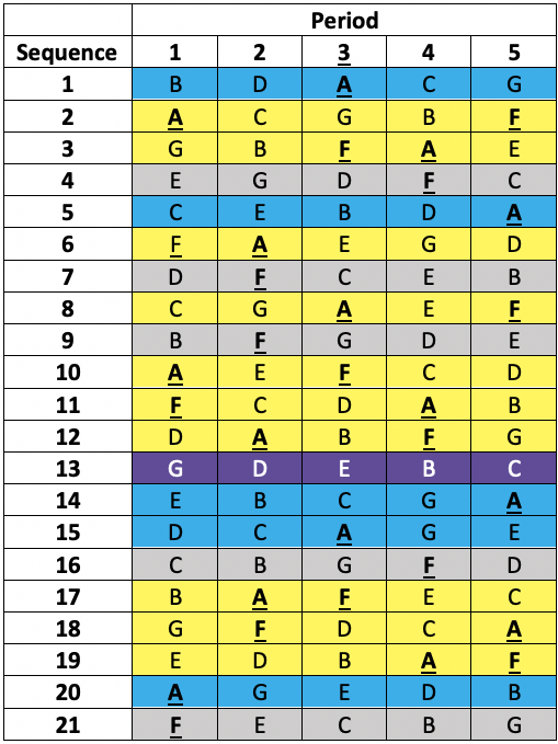
Table 1 Incomplete blocks design in five periods and seven treatments (A to G). Columns are periods, rows are sequences allocated at random to a patient. Yellow: patient received A & F. Blue: patient received A but not F. Grey: patient received F but not A. Purple: patient received neither A nor F.
The active treatments were MTA6, MTA12, MTA24, ISF6, ISF12, ISF24, where the number refers to a dose in μg and the letters to two different formulations (MTA and ISF) of a dry powder of formoterol delivered by inhaler. The seventh treatment was a placebo.
In fact, the plan was to recruit six times as many patients as there were sequences, randomising a given patient to a sequence in a way that would guarantee approximately equal numbers per sequence. This would have given 126 patients in total. In the end, this target was exceeded and 161 patients were randomised to one of the sequences.
Obviously, this is a rather complex design but I have used it because it enabled me to compare two treatments two different ways. First by using only the ten sequences in which they both appear. For this purpose, I could use each patient as his or her control. Second, by using the ten further sequences in which only one appears.
This thus permitted me to analyse data from the same trial using a within-patient analysis and a between-patient analysis. The analyses used above should not be taken too seriously. The analysis would not generally proceed and did not in fact proceed in this way. For example, I ignored the complication of period effects and ignored the fact that by including all the seven treatments in an analysis at once, I could recover more information. I simply chose two treatments to compare and ignored all other information in order to illustrate a point. The two treatments I compared, ‘ISF24’ and ‘MTA6’, were respectively, the highest (24μg) dose of the then (1997) existing standard dry powder formulation, ISF of the beta-agonist formoterol, and the lowest (6μg) of a newer formulation, MTA, it was hoped to introduce. The experiment is discussed in full in Senn, Lilienthal, Patalano and Till11.
The full model analysis that I showed as a dotted line in Figure 1 & Figure 2 fitted Patient as a random effect and Treatment and Period as fixed factors with 7 and 5 levels respectively.
Ed. A link to a selection of Senn’s posts and papers is here. Please share comments and thoughts.


")


I am extremely thankful to Stephen Senn for a further installment on his discussions of randomisation on this blog. His response to the common criticism that RCTs don’t achieve balance is extremely important and opened my eyes to where the critics (often philosophers) go wrong. I would like to draw Stephen out a bit more, though, on what he means in saying randomisation is about randomisation. Fisher said:
The purpose of randomisation . . . is to guarantee the validity of the test of
significance, this test being based on an estimate of error made possible by
replication. (Fisher [1935
b]a1951,psection. 26) (SIST p. 286).The meaning of’ randomisation is about randomisation’, I suggest, is that its function is to guarantee the error probability assessments (for estimators and tests). That is why its relevance comes into question by subjective Bayesians who question the relevance of error probabilities to inference (though some find a role for it in vouchsafing posterior probabilities). For the error statistician, it’s a way to deliberately introduce the probabilistic considerations needed to appraise the reliability of the inference that a method outputs.
Thanks, Stephen, for engaging with our paper and for sharing this convincing argument about the non-necessity of the ‘balance condition’ in RCTs. As you correctly note, we don’t touch upon this in our paper, despite the fact that some arguments for the same statement come also from the philosophy of science front (see for instance J. Fuller, 2018, ‘The Confounding Question of Confounding Causes in Randomized Trials’, Brit. J. Phil. Sci.).
For the point we want to make in our paper, there is no problem to adopt the view that RCT aims to have confounding factors randomly distributed and not homogeneously distributed among groups. In light of your post, we should have said that:
‘…any correlation between the tested intervention and the difference in outcome between the test group and the control group can be estimated, since all other causally relevant factors have been randomly distributed between the two groups’
Rather than what we said, namely that:
‘…any difference in outcome between the test group and the control group should be caused by the tested interventions, since all other differences should be homogenously distributed between the two groups’.
We believe that it would have been technically more correct given what you explain.
For the specific purpose of our analysis in the paper, however, we want to make clear why this is not a misunderstanding of the logic underlying this experimental design.
A quick background. The point in our paper is to argue for the necessity of plurality of methods to make a causal claim in medicine, and it is based on the philosophical idea that what medicine ultimately needs to know about are intrinsic properties (also called dispositions, capacities or causal powers). For instance, Ibuprofen causes gastrointestinal symptoms in a large number of patients. This observation is useful, because it points to an intrinsic property of ibuprofen. Now, whether one agrees with this idea or not, the problem remains that intrinsic properties are not directly observable in the same way that a correlation is, and different methods have some advantages and some blind spots to detect such properties. In the paper, we discuss some of the commonly research methods used in medicine and we explain such advantages and disadvantages for the purpose of detecting intrinsic disposition.
With RCTs, the main point we want to make is that this type of experimental design is the one best suited to detect difference-making at group level, which perfectly fits the Humean definition of causation as difference-maker and regularity. We can say that one randomises for the purpose of having a correspondent degree of variation among and between groups, rather than for the purpose of homogeneity, as argued in the blogpost (to which we have no objection).
This does not change that the aim of randomisation is to make it possible to (1) estimate difference-making, (2) estimate how reliable such estimate of difference-making is.
This is everything we need for what we say in the paper, that:
(1) An estimate of difference-making is a good indication for a disposition, since dispositions tend (although not always do) to make a statistical difference at group level;
(2) Difference-making shows a correlation but not necessarily an intrinsic disposition;
(3) Difference-making might indicate a necessary condition and not an intrinsic disposition.
About this last point, we say:
‘Statistically significant results from an RCT could indicate that the intervention played a causal role for the outcome, either as an intrinsic disposition or as a necessary background condition (a sine qua non). The latter would be where something that was necessary for the effect, although it did not as such cause the effect. Hypothetically speaking, if one had no understanding of the underlying biological mechanisms, one might, for instance, find that hysterectomy significantly reduces the risk of unwanted pregnancy and take this to mean that the uterus is the cause rather than a necessary condition for pregnancy. This shows how what is the advantage of RCTs from a dispositionalist perspective is also the reason why they cannot produce dispositional evidence on their own.’
Elena Rocca and Rani Lill Anjum
Thanks, Elena and Rani Lill. As I said, I find much to agree with in your paper and I am happy to recommend it to others. However,it is perhaps worth my stressing a couple of points again. To contrast n-of-1 trials with randomised clinical trials is not only confusing, since the former are a subset of the latter, but misses, in my opinion, what Fisher was about. Examples where there is randomisation both within and between two levels are rare in clinical trials and it was fortunate that I myself helped to design one and, a quarter of a century later, still had easy access to the data. I was thus able to illustrate directly the point in question.
However, Fisher was used to designing far more complicated experiments with multiple treatments being varied at different levels. The theory he developed to deal with this is already apparent in his 1926 paper and it is also clear that he abandons as unworkable Mill’s idea of equalisation of all nuisance factors. His solution is quite different. He accepts that variation is inevitable and provides a way to estimate it. Thus, in a clinical context, his theory applies not only to parallel group trials but to cluster randomised trials, cross-over trials, incomplete block trials and n-of-1 trials.
I also wish to point out to one distinction that is important. The theory distinguishes between treatment factors and blocking factors. The latter are the province of nature and their effects are simply accepted as a fact of life to deal with. The purpose of the experiment is to estimate the effects of the treatment factors and this purpose is indeed causal, even if the causality is not studied at a fundamental mechanistic level. This distinction is absolutely fundamental and reflected in John Nelder’s theory, which may be regraded as the apotheosis of Fisher’s, and which provide a calculus of experiments whose power and scope deserve to be more widely known and understood.(See https://errorstatistics.com/2018/11/11/stephen-senn-rothamsted-statistics-meets-lords-paradox-guest-post/ )
Stephen:
In their comment, Elena Rocca and Rani Lill Anjum suggest:
“In light of your post, we should have said that:
‘…any correlation between the tested intervention and the difference in outcome between the test group and the control group can be estimated, since all other causally relevant factors have been randomly distributed between the two groups’”
I wonder if you agree with this, or might you put it something like the following: We can use the observed difference in effect (between treated and controls) to estimate the effect(s) due to the treatment (along with its reliability), because we have randomly assigned subjects (to T or C).
The randomization introduces probability into the analysis (no probability in, no probability out.). If the the treatment makes no difference, we can assess the probability of the observed difference occurring by the random assignment into groups. Much of my understanding of randomization, of course, comes from you and David Cox. (I’m using the “z” spelling).
I would have avoided, myself, to use the word “correlation”, which Elena Rocca and Rani Lill Anjum used. The purpose of randomised clinical trials, whether parallel, cluster, cross-over or n-of-1 is, indeed, causal.
Thus, randomisation is a device for enabling us to make precise estimates of an inevitable imprecision.I think, Prof. Stephen Senn gives a very stunning argument of randomization in the whole blog, but in the end, his argument is not correct by stating ” make precise estimates of an inevitable imprecision”. Instead, it may be “make estimates of an inevitable imprecision reliable” because balance is a matter of precision but randomization can not guarantee balance and precision.
I agree with Ning Li, Stephen’s post is great but the use of “precise” at the end is not quite right. I like to tell students that the randomisation (Australian ‘s’) is necessary to allow _calibrated_ statements about the imprecision.
I always love Stephen’s posts!
Just in case anyone is interested, there’s intriguing work by Donald Rubin and co-workers on “re-randomisation”, meaning that if randomisation leads to a too unbalanced sample (in terms of one or more covariates), it is discarded and the sample is randomised again. As far as I can see, this preserves all positive features of randomisation and makes it more precise (with somewhat more difficult theory behind it).
Key references are
K. L. Morgan and D. B. Rubin. Rerandomization to improve covariate balance in experiments.The Annals of Statistics, 40:1263–1282, 2012.
K. L. Morgan and D. B. Rubin. Rerandomization to balance tiers of covariates.Journal of the American Statistical Association, 110:1412–1421, 2015.
Dear Christian,
Thanks. I have not read this and must look it up. However, randomisation in clinical trial is a sequential, dynamic and ongoing activity: patients are assigned to treatment when or shortly after, they present, As I often put it, we have little if any control over the presenting process but have tight control of the allocation algorithm. Thus, I don’t think that re-randomisation can often be a possibility, but perhaps I have misunderstood.
Stephen:
But the goal of their re-randomization I thought was to achieve balance which you say is not needed. In taking a random sample, by contrast, Fisher will say it’s fine to have a do-over if it is very skewed, right?
Balance is not needed for the theory to apply and for randomisation to achieve what the theory states it achieves. However, that doesn’t rule out that you can get more precision with improved balance.
A lot of attention has been given to the recent attempt to estimate the proportion of people with antibodies to covid-19 in Santa Clara county, California–seroprevalence, as it is described–using sample that are intended to be “balanced. This moves us a little away from the direct topic of Senn’s post(though not more so than the usual flow of discussions on this blog), which is why I held it back until today, I would be extremely interested in knowing what Stephen, and others, think of this, and especially the report of CIs. The same methodology is being used elsewhere. I’m not sure the existing criticisms are getting at the main issues, and it will be important to make improvements.
The study is laid out pretty clearly in the article. It seems obvious enough that there are people out there who have had it and are not documented because of the rationing of tests, because of asymptotic people, and because cases are still increasing.
I think testing for antibodies is extremely important and I’m glad we’re starting to increasingly see it (there is an NIH site now to volunteer). I just don’t see why a random sample isn’t done, at least of a given city or state. Here’s what the Stanford people did (one of a multitude of authors is Ioannidis). The link is below.
“Participants were recruited using Facebook ads targeting a representative sample of the county … We report the prevalence of antibodies to SARSCoV-2 in a sample of 3,330 people, adjusting for zip code, sex, and race/ethnicity.
…The unadjusted prevalence of antibodies to SARS-CoV-2 in Santa Clara County was 1.5% (exact binomial 95CI 1.11-1.97%), [50 of 3330 in the sample] and the population-weighted prevalence was 2.81% (95CI 2.24-3.37%).
Under the three scenarios for test performance characteristics, the population prevalence of COVID-19 in Santa Clara ranged from 2.49% (95CI 1.80-3.17%) to 4.16% (2.58-5.70%).
These prevalence estimates represent a range between 48,000 and 81,000 people …, 50- 85-fold more than the number of confirmed cases”.
I wasn’t sure if the study precluded subjects who either tested positive for covid-19, or who were told, “your symptoms are entirely in keeping with covid-19 patients, but we are only allowed to test patients in hospitals, so proceed with the following at-home care”. This is the case in NYC, and those patients were often treated with medicines but at home. As I read the paper, and its indications of possible biases, it appears that such people were NOT precluded from this study. Yet it stands to reason that people who tested positive or who were told they almost certainly have it would been the most keen to be tested for antibodies. That would bias the sample.
It would be interesting to know what % of the people tested reported having symptoms (in answer to that question).
A concern that I would have is the “adjusted” measure of seroprevalence from 1.5% to around 3% or more. I’m sure they didn’t predesignate the adjustment technique, although it’s partly explained in the article.
I’m sure all this will get corrected soon.
Click to access 2020.04.14.20062463v1.full.pdf
Gelman reviews some of the criticisms of the study here:
https://statmodeling.stat.columbia.edu/2020/04/19/fatal-flaws-in-stanford-study-of-coronavirus-prevalence/
On a rough scan of his blog, a key problem is that using the lower estimate of specificity (essentially the complement of the type i error) would produce an interval that included 0.
Some of his points are:
“you’d want to record respondents’ ages and symptoms. And, indeed, these were asked about in the survey. However, these were not used in the analysis and played no role in the conclusion. In particular, one might want to use responses about symptoms to assess possible selection bias”.
…I’m concerned about the poststratification for three reasons. First, they didn’t poststratify on age, and the age distribution is way off! Only 5% of their sample is 65 and over, as compared to 13% of the population of Santa Clara county.”
… once the specificity can get in the neighborhood of 98.5% or lower, you can’t use this crude approach to estimate the prevalence; all you can do is bound it from above, which completely destroys the ’50-85-fold more than the number of confirmed cases’ claim.”
Here’s a copy of a letter (toward bottom of article) sent out to advertise the study which tells people that participating will give them piece of mind by indicating if they are now immune. Of course this would bias the test toward people who believe they’ve been infected. Other problems with the way it was advertised are noted in this article.
https://www.buzzfeednews.com/amphtml/stephaniemlee/stanford-coronavirus-study-bhattacharya-email?__twitter_impression=true
All I can take away from the Santa Clara county study is that the level of penetrance of COVID19 is low within that population (apparently under 10%), and is nowhere near any level at which herd immunity might occur. Additionally, reported COVID19 case counts available in newspapers or the Johns Hopkins website are obviously undercounts, as they report only ‘confirmed cases’ and associated deaths, and the orchestrated lack of testing keeps those counts artificially lower.
There are indeed problems with the sample of convenience obtained via Facebook, and resultant bias remains unknown. Arguing over whether the penetrance rate is 1.5% or 4% or 0% seems a distraction. Hopefully some group of researchers will conduct a better population-level random sample assessment to get an unbiased read on COVID19 penetrance. One method we still currently possess to allow reaching something more closely resembling a truly randomly sampled set is the US Postal Service, which has access to far more households than land line telephones (too many old people), cel phones (too many young people), or Facebook users (too many tech-savvy wealthier people). Invitations for screening delivered by mail will reach a more representative population sample set.
Steven:
Great idea! Maybe that would help prevent the postal service from going bankrupt! Today, it was announced that an antibody test in NY estimated around 20% in NYC were exposed/infected. I’ll add the link.
The USPS would not look like it was going bankrupt if congress had not legislated that it pre-pay employee retirement and health benefits far into the future, unlike any other public or private business.
https://about.usps.com/who-we-are/financials/annual-reports/fy2010/ar2010_4_002.htm
Just saying…
Michael: You keep up with the U.S. postal service?
I like to keep up with the big lies that drive America. One of those is that the USPS is unable to cover its costs. Another is that it would be a good thing that the USPS be closed or sold off.
I’m not a political scientist and I’m not a social scientist, but American politics and American society offer lessons for anyone who likes to see.
(Don’t drink disinfectant.)
Thank you Stephen Senn for setting the record straight on “N of 1” trials. They are indeed a subset of randomized trials, in the subcategory of blocked designs, which go back decades. When I first started my statistical studies in the 1970s, such designs were known in the statistics community as blocked designs. Somewhere in the 1980s medical personnel ‘rediscovered’ such analytic procedures and termed them “N of 1” studies.
I am always suspicious of relabeled designs, as the subsequent hyping of the new label often seems more of a marketing campaign than serious scientific effort. One stark example was the labeling and hyping of gene subsets identified via straightforward principle components or singular value decomposition methods by the Duke group including Nevins and Potti a decade ago. The subsets were labeled ‘supergenes’ then ‘metagenes’ (a patent applied for on that one) then ‘gene expression signatures’ – we all know now how that marketing effort worked out.
Another example I find irksome is the “Allred score” used by pathologists, a brain-dead combination of tissue sample staining intensity score (0, 1, 2 or 3 depending on how dark the stain appears under the microscope) and percentage of cells that show the staining, reducing two measures to one dimension via a formula that seems ‘mathy’ and has the name of a charismatic researcher and a citation that can be added to journal articles.
Here Stephen Senn reminds us that “N of 1 studies” are nothing more than randomized block designs, and demonstrates beautifully in Figure 1 why the paired t-test for a blocked design can be superior to the unpaired t-test in a non-blocked design, even when the unblocked design has twice as many subjects as the blocked design. When within-blocks correlation is high the loss of degrees of freedom for a test statistic is far outweighed by the reduction in variability achieved via blocking.
The moniker “N of 1 study” just sells better than “randomized block design”, especially in this age of “personalized medicine” (when was medicine ever not personal?) so the label will be with us for a while yet, until some new charismatic researcher comes up with an even trendier label. The problem with this phenomenon is that non-statisticians end up thinking that the newly labeled method is somehow different from its original methodological family, and the newly labeled method gets its own rows in tables, its own separate discussion in papers, as happened here with science philosophers Rocca and Anjum.
Thankfully we have sensible statisticians such as Stephen Senn to reinject a dose of reality and scientific professionalism in these situations, reminding us all about the value of blocking and how to properly analyse data from such designs, regardless of their current trendy moniker.
Re randomisation is an issue in many applications areas, not so much in clinical trials. Part of the difficulty is with hard to change factors. Obviously if this is accounted ab initio one can design the experiment accordingly. David Cox, in his 1958 book on planning of experiments, deals with this. He provides 3 approaches to it. One is to account, ahead of time, for allocation patterns that are not feasible, in practice’ leading to restricted randomisation.
The way I have looked at this is through the generalisation prism. If you randomize and get AAAAAABBBBB, your treatment effect findings will be difficult to justify since a confounding time effect cannot be ignored, thus impacting the findings’ generalisation. All this has been presented in various seminars and workshops on causality I delivered and, if anyone is interested, I will be glad to share the slides.
Strangely enough, Fisher never wrote about re-randomization. However, as mentioned by Mayo, he did have a pragmatic approach and, given an unjustifiable allocation , would leave the room and return with a different allocation (testimonial of Cochran related to Don Rubin). My add on is that the term “unjustifiable” means, poor generalisability. As some of you know, generalisability is the 6th information quality dimenstions (See my book with Gality Shmueli on information quality, Wiley, 2016).
Re-randomisation has been proposed by a number of philosophers but although possible in agriculture where you have a static field with known plots and subplots to which you will allocate treatment it can’t be done in a clinical trial, since patients have to be treated sequentially when they present. There is no going back in time to reallocate and you don’t know who will be in your trial until they have arrived. See Myth 1 of Seven myths of randomisation in clinical trials https://onlinelibrary.wiley.com/doi/abs/10.1002/sim.5713 .
The time effect that you mention is one of the exceptions. There is a theory of restricted randomisation. Usually it tries to keep first and second moments OK but (IMO) the net effect will be that some of the higher order moments are affected. (This probably doe not matter too much.) Rosemary Bailey is an expert on this sort of thing.
Stephen
As I wrote, re-randomisation is a realistic issue in several application domains, such as industrial applications, but as you also stress, apparently not in clinical trials. However, I wonder if there are no example like this where the randomized allocation is tampered by doctors or health care providers. Properly blinding the study is of course essential, but is it always done properly?? On the humorous slide of placebo effects you might have seen https://www.youtube.com/watch?v=vklzzTI3VwI
The two points my comments above aimed at are::
1. Why is this a problem
2. If it is a problem, how can you handle it
Regarding (1) allocations through randomization that produce difficulties in generalisation of findings are a serious problem. If you remain aestenistic and use, through randomization, allocation patterns which cannot generalise the findings you will have issues with communication of your findings. To me this is a reflection of poor information quality.
Regarding (2) as mentioned, Cox (1958) adresses the issue and present three scenarios. If you block what you can, account for hrd to change factors in the experimental design and identify ahead of time allocations you want to exclude, the analysis can handle that (e/g/ REML). If you do not do that and “play by the ear” your analysis will be problematic which, again, will be reflected by poor information quality.
The problem of course is that the best time to properly design an experiments is after you finished running it.
The only connection I see with randomisation and generalisation is the following. Randomisation helps us tackle the causal task of establishing treatment effects in the patients actually studied. Establishing that is a sort of minimal task on the road to then predicting the treatment effect more generally. Obviously, if we get this first step wrong, we are likely to get further inferences wrong also. However, this further step itself (really more of a leap) has more to do with matters such as choosing an appropriate scale to transfer effects and judgement as to the relationship between the patients actually studied and those to whom one wishes to establish effects. The randomisation does not help with this further step in itself. See https://onlinelibrary.wiley.com/doi/10.1002/sim.2074
Stephen – thank you for the note and reference, Indeed randomisation “is valuable in increasing the credibility of inferences drawn from clinical trials.”. In the language of Pearl it “mutilates” the DAG, some sort of pseudo do calculus. Now, generalisation “a la Pearl” would get you to transport findings in A to set up B. For example. generalise findings from a clinical trial in population A to population B, I suggest that randomisation will help you, in using a DAG account for population covariates. So that, beyond “increasing the credibility” , it enhances generalisability. This might also be a question for philosophers to address….
Ron: Philosophers have addressed it and it’s a main reason so many of them are critical of RCTs. But, as Senn emphasizes, their function is to estimate the causal effect in the subjects (or experimental pop). If the experimental pop is also a random sample from pop B, then it can be generalized. But the knowledge gained is still (generally!) going to be relevant for making inferences about other pops, even if it’s to understand why it would be wrong to generalize to pop B. (e.g., giving nutritional info to mothers may be shown to improve family health in developing pops where women shop, but it’s no surprise the effect doesn’t show up in places where only men shop). Or the like.
(This kind of criticism is common in RCT4Dev Econ).
David Cox, in a workshop we held a decade ago at the LSE, which also included Senn, hammered this point in response to skepticism by Cartwright and Worall. Website:
https://www.phil.vt.edu/dmayo/conference_2010/index.htm
The very fact the subjects volunteer, he points out, may make them different from others.
But, as Cox argues, it is a mistake to see this as grounds to reject, or fail to appreciate, the great power of RCTs–at least when they can be done, and doing so is relevant.
There was little doubt that the results from RCTs on hormone replacement therapy in early 2000s (it does not prevent age-related diseases & it increases risks of heart disease) were relevant for the general population of women. Prescribing practice changed overnight! (For years there was resistance to even doing an RCT because the medical profession was so certain of its benefits! It took years of pressure by various women’s groups to finally get them.)
The fact that what was learned also resulted in finding out about subgroups, and altered types of HRTs, that may avoid the harms, in no way shows a problem with the RCTs–quite the opposite. They figured out where to look, and how to change practice only thanks to the RCTs*.
*Steven Goodman finally admitted this was so, when I raised it in a panel we were in recently (remember when we used to attend conferences?) He told the group, ‘it turns out that we could have found the same results they found in the RCTs using our observational studies!’ I pointed out that they only learned how to find what the RCTs found thanks to the RCTs. Before that, due to “healthy women’s syndrome”, and other biases, HRTs appeared universally beneficial for postmenopausal women. He admitted, ‘yes, of course, she’s right, we found them only because of the RCTs’. But he still touts non-RCTs.
I agree. There are various defences that can be made of concentrating on the local causal effect and regarding this as an important task to get right with generalisation being a secondary task. One is that main effects (confounding) are generally more important than interactions (effect modification). (Here the terms in brackets are those used by epidemiologists.) The idea that higher order interactions are progressively less important than lower ones is key to the design of fractional factorial experiments. RCTs are good at dealing with confounding, not because confounders are eliminated but because their joint effect can be estimated. This is valuable. The second is that the combination of a well-estimated effect on an additive scale, together with further information, can be a (fairly) successful way to predict on a relevant scale. This idea is discussed here. https://www.slideshare.net/StephenSenn1/real-world-modified Finally, one should not let the perfect become the enemy of the good. Of course the effect in the trial is not guaranteed to predict perfectly what one would see in the population. However, estimating it well is a very useful first step.
Stephen:
You really put your finger on the essential point, so often missed: “RCTs are good at dealing with confounding, not because confounders are eliminated but because their joint effect can be estimated. This is valuable.” Being able to estimate their joint effect enables an estimate of the treatment effect that is not biased by confounding. I think that philosophers, trained on “confirmation theory”, overlook this essential logic of (what I would call) learning from error. To explain this (often circuitous) logic is the arduous task of my book: SIST.
Today we heard results from two RCTs on a covid drug, remdesivir, that are in some tension with each other. The published study in the lancet:
Click to access remdesivir-in-adults-with-severe-covid-19-a-randomised-double-blind-placebo-controlled-multicentre-trial-1.pdf
(from China) showed no statistically significant decrease in days to recovery or mortality, but it was deemed too small. That’s because they said they had trouble enrolling in China since there weren’t enough patients with covid-19. (It also failed to show a significant reduction in viral RNA in those treated.)
But Dr. Fauci gave an extremely optimistic report on a review of results in an NIH adaptive, randomized trial. In this study, there was a statistically significant decrease in days to recovery (11 vs 15). Fauci announced it as the new standard of care. He said it was “showing a trend” toward reduced mortality but was not statistically significant “yet”. By declaring remdesivir the new standard of care, however,the placebo patients were or are to be given it, so no assessment of mortality reduction can be made (as I understand it). It is said to be “trending” towards significance.
https://www.nih.gov/news-events/news-releases/nih-clinical-trial-shows-remdesivir-accelerates-recovery-advanced-covid-19
I, like everyone else, will be jumping for joy if they’ve made any progress on treatment. But isn’t it odd that Fauci didn’t mention the Lancet study (or maybe I missed it)? Should they have waited for the mortality results of the NIH study before declaring it the standard of care?
https://arstechnica.com/science/2020/04/first-treatment-for-sars-cov-2-shortens-recovery-time/
The study that Fauci was taking about is NCT04280705, Lancet paper is describing NCT04257656
How very odd it is to describe a static number as a “trend toward significance”!
Thanks for the great post,
Simple question from a non-statistician regarding your statement below:
“can we estimate how reliable they are?’. The answer he provides is ‘yes’ if we randomise”,
What does that mean for non-randomized studies, for example when estimating treatment effects and the uncertainty around using CI
I know that this is an old post, but a workshop on foundations of randomisation is coming next week and hat remindd me of it. I re-read it and I am still wondering how this view, that randomisation is not aimed to homogenisation, fit with the practice of baseline assessment. I thought that it consists on checking whether some chosen parameters are equally similarly distibuted in the two groups. In the words of Sackett et al 1997, it is a ‘double check to see whether the randomisationwas effective by looking to see whether patients were similar at the start of the trial’. Is baseline control checkng whether they are randomly distributed instead? And how would one check random distribution, if not by comparing the distribution within and between the two groups?
Thanks for the comment.
As I explained, balance is not necessary for valid inference. Also, balance does not guarantee valid inference. Consider a randomised block design (the blocks might be centres or, in a within-patient study, patients). If the design is perfectly balanced by block, then the block effect has been eliminated by design from the treatment estimate. It will make no difference to the estimate (for a linear model) whether you fit it or not. However, if the block effects are predictive (which is presumably why the design was blocked) then the standar error will be different if the block is fitted to if it is not. Which is correct? The answer is the analysis that fits block effects. Since these have no effect on the estimate (because of the design) it would be wrong if their variation were allowed to contribute to the estimate of the error of the estimate.
On the other hand consider a factor that it is not prognostic but that is imbalanced. Clearly it can have no effect on the estimate so that it can be ignored.
In other words, examining factors for balance is no part of a rational strategy for analysis. If we are so unsure as to whether a factor should be in the model or not, the only way to see whether it makes any difference is to put it in the model and see. Anything else just avoids the issue.
All of this is discussed in greater detail in https://onlinelibrary.wiley.com/doi/abs/10.1002/sim.5713
Pingback: Study Reports Covishield 63% Effective Against Delta. The Devil’s in the Details. | hi INDiA