

Excursion 3 Exhibit (i)
Exhibit (i) N-P Methods as Severe Tests: First Look (Water Plant Accident)
There’s been an accident at a water plant where our ship is docked, and the cooling system had to be repaired. It is meant to ensure that the mean temperature of discharged water stays below the temperature that threatens the ecosystem, perhaps not much beyond 150 degrees Fahrenheit. There were 100 water measurements taken at randomly selected times and the sample mean x computed, each with a known standard deviation σ = 10. When the cooling system is effective, each measurement is like observing X ~ N(150, 102). Because of this variability, we expect different 100-fold water samples to lead to different values of X, but we can deduce its distribution. If each X ~N(μ = 150, 102) then X is also Normal with μ = 150, but the standard deviation of X is only σ/√n = 10/√100 = 1. So X ~ N(μ = 150, 1).
It is the distribution of X that is the relevant sampling distribution here. Because it’s a large random sample, the sampling distribution of X is Normal or approximately so, thanks to the Central Limit Theorem. Note the mean of the sampling distribution of X is the same as the underlying mean, both are μ. The frequency link was created by randomly selecting the sample, and we assume for the moment it was successful. Suppose they are testing:
H0: μ ≤ 150 vs. H1: μ > 150.
The test rule for α = 0.025 is:
Reject H0: iff X > 150 + cασ/√100 = 150 + 1.96(1)=151.96,
since cα = 1.96.
For simplicity, let’s go to the 2-standard error cut-off for rejection:
Reject H0 (infer there’s an indication that μ > 150) iff X ≥ 152.
The test statistic d(x) is a standard Normal variable: Z = √100( X – 150)/10 = X – 150 which, for x = 152 is 2. The area to the right of 2 under the standard Normal is around 0.025.
Now we begin to move beyond the strict N-P interpretation. Say x is just significant at the 0.025 level (x = 152). What warrants taking the data as indicating μ > 150 is not that they’d rarely be wrong in repeated trials on cooling systems by acting this way–even though that’s true. There’s a good indication that it’s not in compliance right now. Why? The severity rationale: Were the mean temperature no higher than 150, then over 97% of the time their method would have resulted in a lower mean temperature than observed. Were it clearly in the safe zone, say μ = 149 degrees, a lower observed mean would be even more probable. Thus, x = 152 indicates some positive discrepancy from H0 (though we don’t consider it rejected by a single outcome). They’re going to take another round of measurements before acting. In the context of a policy action, to which this indication might lead, some type of loss function would be introduced. We’re just considering the evidence, based on these measurements; all for illustrative purposes.
Severity Function:
I will abbreviate “the severity with which claim C passes test T with data x“:
SEV(test T, outcome x, claim C).
Reject/Do Not Reject: will be interpreted inferentially, in this case as an indication or evidence of the presence or absence of discrepancies of interest.
Let us suppose we are interested in assessing the severity of C: μ > 153. I imagine this would be a full-on emergency for the ecosystem!
Reject H0. Suppose the observed mean is x = 152, just at the cut-off for rejecting H0:
d(x0) = √100(152 – 150)/10 = 2.
The data reject H0 at level 0.025. We want to compute
SEV(T, x = 152, C: μ > 153).
We may say: “the data accord with C: μ > 153,” that is, severity condition (S-1) is satisfied; but severity requires there to be at least a reasonable probability of a worse fit with C if C is false (S-2). Here, “worse fit with C” means x ≤ 152 (i.e., d(x0) ≤ 2). Given it’s continuous, as with all the following examples, < or ≤ give the same result. The context indicates which is more useful. This probability must be high for C to pass severely; if it’s low, it’s BENT.
We need Pr(X ≤ 152; μ > 153 is false). To say μ > 153 is false is to say μ ≤ 153. So we want Pr(X ≤ 152; μ ≤ 153). But we need only evaluate severity at the point μ = 153, because this probability is even greater for μ < 153:
Pr(X ≤ 152; μ = 153) = Pr(Z ≤ -1) = 0.16.
Here, Z = √100(152 – 153)/10 = -1. Thus SEV(T, x = 152, C: μ > 153) = 0.16. Very low. Our minimal severity principle blocks μ > 153 because it’s fairly probable (84% of the time) that the test would yield an even larger mean temperature than we got, if the water samples came from a body of water whose mean temperature is 153. Table 3.1 gives the severity values associated with different claims, given x = 152. Call tests of this form T+

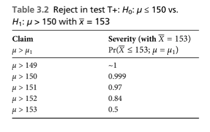
In each case, we are making inferences of form: μ > μ1 = 150 + γ, for different values of γ. To merely infer μ > 150 , the severity is 0.97 since Pr(X ≤ 152; μ = 150) = Pr(Z ≤ 2) = 0.97. While the data give an indication of non-compliance, μ > 150, to infer C: μ > 153 would be making mountains out of molehills. In this case, the observed difference just hit the cut-off for rejection. N-P tests leave things at that coarse level in computing power and the probability of a Type II error, but severity will take into account the actual outcome. Table 3.2 gives the severity values associated with different claims, given x = 153.
If “the major criticism of the Neyman-Pearson frequentist approach” is that it fails to provide “error probabilities fully varying with the data” as J. Berger alleges, (2003, p.6) then, we’ve answered the major criticism.
Non-rejection. Now suppose x = 151, so the test does not reject H0. The standard formulation of N-P (as well as Fisherian) tests stops there. But we want to be alert to a fallacious interpretation of a “negative” result: inferring there’s no positive discrepancy from μ = 150. No (statistical) evidence of non-compliance isn’t evidence of compliance, here’s why. We have (S-1): the data “accord with” H0, but what if the test had little capacity to have alerted us to discrepancies from 150? The alert comes by way of “a worse fit” with H0–namely, a mean x > 151*. Condition (S-2) requires us to consider Pr(X > 151; μ = 150), which is only 0.16. To get this, standardize X to obtain a standard Normal variate: Z = √100(151 – 150)/10 = 1; and Pr(X > 151; μ = 150) = 0.16. Thus, SEV(T+, x = 151, C: μ ≤ 150) = low(0.16). Table 3.3 gives the severity values associated with different inferences of form: μ ≤ μ1= 150 + γ, given x = 151.
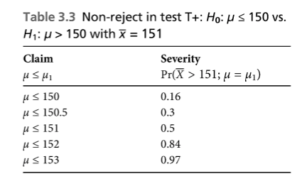
Can they at least say that x = 151 is a good indication that μ ≤ 150.5? No, SEV(T+, x = 151, C: μ ≤ 150.5) ≅ 0.3, [Z = 151 – 150.5 = 0.5]. But x = 151 is a good indication that μ ≤ 152 and μ ≤ 153 (with severity indications of 0.84 and 0.97, respectively).
You might say, assessing severity is no different from what we would do with a judicious use of existing error probabilities. That’s what the severe tester says. Formally speaking, it may be seen merely as a good rule of thumb to avoid fallacious interpretations. What’s new is the statistical philosophy behind it. We no longer seek either probabilism or performance, but rather using relevant error probabilities to assess and control severity.5
5Initial developments of the severity idea were Mayo (1983, 1988, 1991, 1996). In Mayo and Spanos (2006, 2011), it was developed much further.
***
NOTE: I will set out some quiz examples of severity in the next week for practice.
*There is a typo in the book here, it has “-” rather than “>”
You can find the beginning of this section (3.2), the development of N-P tests, in this post.
To read further, see Statistical Inference as Severe Testing: How to Get Beyond the Statistics Wars (Mayo 2018, CUP).
Where you are in the journey:
Excursion 3: Statistical Tests and Scientific Inference
Tour I Ingenious and Severe Tests 119
3.1 Statistical Inference and Sexy Science: The 1919
Eclipse Test 121
3.2 N-P Tests: An Episode in Anglo-Polish Collaboration 131
YOU exhibit (i) N-P Methods as Severe Tests: First Look (Water Plant Accident)
3.3 How to Do All N-P Tests Do (and more) While
a Member of the Fisherian Tribe 146


")


At some point I remember S1 being stated as something like:
> There is a high probability of getting as good a fit or better under H0.
Rather than just ‘there is a good fit’
So
S1 is a high prob of so good a fit or better under H0
S2 is a high prob of a worse fit under HA
Has this changed at some point or do I misremember?
(The version I’ve stated is also closer to Birnbaum’s, other than yours being post data)
Thanks!
Yes SEV is post data.
Just to clarify – I’m asking about the two conditions S1 and S2.
It would seem natural to require not just a good fit for S1, but a good fit with high probability.
Eg if H0 fits the data by fluke and H1 fits worse with high prob then has H0 really passed a severe test?
Surely one would also want H0 to reliably fit?
Do you mean high prob under Ho? you don’t want a high prob of good fit with false hyp. But the former must be qualified. some might want comparatively good fit. the sig tester wants Pr(d < do;H0) = high (1 – p)
I just mean I want to make the two severity requirements S1 and S2 both refer to the probability of fit under different hypotheses, instead of just S2.
Eg
S1: H produces a good fit to y with high probability
S2: Alternative Ha produces a worse fit to y with high probability
Does that make sense?
Or am I missing something subtle here re: the meaning of H and/or ‘fit’?
We need to distinguish the pre-data error probabilities associated with a good test statistic or distance measure, and what is said post data. In considering a claim C of interest, one wants to know the probability the method would have resulted in finding a flaw (by dint of a worse fit) were C false (or a given flaw present).
I intend the general requirement to be fleshed out for the case at hand, yet I don’t want to preclude applying the requirement to critically evaluate other approaches. Were I staying just within the error statistics of a Fisher or N-P, I’d more directly use the notions within. Why don’t you see what you think of FEV–the ‘frequentist notion of evidence’ I articulated with Cox.
I mean you use:
S1: H fits data
S2: with high probability, Ha does not fit as well
Why not:
S1: with high probability, H fits data
S2: with high probability, Ha does not fit as well
Since in my mind, H specifies a probability model, the above would make more sense to me.
Roughly S1 relates to the realised Type I error and S2 the realised Type II error.
What do you think?
I think I responded.If we speak of a high prob of H fitting, it would have to be under H.
Yeah, comment was stuck in void.
They are slightly less precise than they should have been. Meant to say:
S1: there is a high prob of an as good or better fit with H, under H
&
S2: there is a high prob of a worse fit with H, under HA
Spoze, to start, Ho is rejected in a 1-sided test w/ low p-value, & evidence of HA inferred. Pr(worse fit w/ HA; Ho) = 1 – p.
Since our claim is ‘HA’.
Do you also want to consider
S1’: Pr(better fit w/ HA; HA) high
here?
So here the claim is HA.
So I’m thinking we should consider both:
S1: There is a high probability of getting as good a fit or better with HA than that observed, under HA.
S2: There is a low probability of getting as good a fit or better with HA than that observed, under H0.
No?
In this case, the “severity” is just the Bayesian posterior probability (with the usual flat prior on the location parameter) of the corresponding interval.
It would be instructive to see an example where this correspondence doesn’t occur, to be able to compare the two approaches.
Agreement on numbers doesn’t get rid of important disagreements in interpretation. This section is not comparative, but read the rest of the book
The readings are i.i.d. double exponential centred at 150 with standard deviation 10.
H_0: mu150 where mu is the centre of symmetry.
The test rule for alpha=0.025 is
reject H_0 if X_med > 150+0.106*10*sqrt(2)=151.5
This is more severe than your proposal. Why don’t you use it?
Hi Laurie,
So let me see if understand your question.
You’re asking:
– Same data, same alpha, different beta/SEV, different models.
– The second model has better alpha and beta/SEV
So why not use the second model?
And presumably your intended answer is that the second model ‘imports severity’?
I’ve no clue how you’re using ‘a model imports severity’, except maybe if you change the assumptions of the question, you can solve a different problem more severely.
Should read
H_0: mu150 where mu is the centre of symmetry
Try again in words
H_0: mu less than or equal to 150 vs. H_1 mu greater than 150 where mu is the centre of symmetry
Oliver, exactly. Models import severity. In Tukey’s words TINSTAAFL, there is no such thing as a free lunch, at least not in statistics. If you develop a theory of severity you have to take this into account. As far as i see Mayo does not do so and her theory therefore has a large gap. The ‘solution’ is almost an oxymoron, for severity use the least severe model.
Laurie: I may have missed a round, but what is this gap resulting in an oxymoron for severity?
Deborah, the problem is the one you described at the beginning, 100 measurements of water temperature etc. You then write that each measurement is like observing X~ N(150,10^2). Depending on what you mean by ‘like’ each measurement could also be like observing X~Laplace(150, 10/sqrt(2)) . In each case you identify the centre of symmetry of the distribution, here 150, with the temperature. Given each model you want to be severe which leads to the optimal estimator of the mean in the Gaussian case and the median in the Laplace case. It turns out, as to be expected, that for a given alpha here 0.025 the Laplace model allows you to detect smaller differences than the Gaussian, 151.5 as against 152.
It would at first sight seem that if you want to determine the temperature as accurately as possible you should use the Laplace model. The increase in severity comes at no cost, you just change the model. Tukey calls it a free lunch. The severity of your procedure depends on the model you are using assuming that you use the optimal estimator for the model. You may object that given 100 observations you can distinguish between the Gaussian and Laplace models. This doesn’t help. I could take a mixture model say 0.5N+0.5L such that you can’t distinguish. The mixture model will again be more severe than the Gaussian. What to do?
Importing severity through your choice of model could be seen as not being honest. To be honest you should choose that model which is least severe. Severity can be measured asymptotically by 1/F where F is the Fisher information., the larger F the more severity you have imported. Thus to be honest you should not maximize F for maximum severity but minimize F for minimum severity. In the location problem it if the Gaussian distribution which minimizes it, it is the least severe distribution. So with certain caveats I will not go into your choice of the Gaussian model was correct but your justification for this cannot simply be ‘each measurement is like observing X~ N(150,10^2)’. It goes deeper than this. We have discussed this once before using my example of copper in drinking water.
On a mathematical level using a model with an optimal estimator is ill posed because one has optimal=maximum likelihood at least asymptotically. Likelihood = density =differentiation= an unbounded inverse. You therefore have to regularize. Minimum Fisher information is a form of regularization. None of this is new, it is all well known in the robustness community.
Hi Laurie,
“You then write that each measurement is like observing X~ N(150,10^2). Depending on what you mean by ‘like’ each measurement could also be like observing X~Laplace(150, 10/sqrt(2)) ”
true, but Mayo is assuming the Normal model holds in this example, and has invoked the Central Limit Theorem.
In her book “Statistical Inference as Severe Testing”, Mayo has suggested that severity can be defined in a nonparametric manner, which would be more general, but probably harder to follow/calculate than using familiar normal distribution theory,
Thanks,
Justin
http://www.statisticool.com
Yes. My book takes as its guide the statistics wars now being debated. If you study them, you will find them revolve around the examples I give: generally Normal distributions with known sigma. Jim Berger set the example, explaining, quite rightly in my opinion, that if we can’t first get clear about the very simple cases, it will be harder to get at the crux of the matter with more complex cases. I agree that more should be made about testing assumptions, and I devote some discussion to that problem. In any event, one can’t talk about everything at once, and here I’m just introducing the notion.
Mayo:
Unfortunately once you get the simple case sorted you (or someone) need(s) to move on to less simple ones. That takes someone into Laurie’s territory where doubly unfortunately simple cases are often a bad guide.
Keith O’Rourke
A bad guide to what? Please explain.
The goal of the book is to get us beyond today’s statistics wars, and while I can’t deal with all of them, I do deal with the main ones. Today we have people arguing that we need to “redefine” statistical significance so that P-values fall into line with Bayes factors or other numbers. Many who approve aren’t keen to do inference by way of Bayes factors. So why are they judging error statistical methods by means of standards from an account that may not block tests that lack severity. If you ask the 70-odd people who signed on if they would countenance the Bayesian method + diagnostic testing employed in that paper, few will say yes (I haven’t come across any). I haven’t My goal in the book is to faciltate the critical analysis of these debates which may well leave us with “reforms” that won’t improve science at all.
If Laurie is concerned with other problems that threaten and confuse statistical practitioners, I hope he will write about them.
The hardest thing one finds in writing a book like this is just how difficult it is to say any thing at all. Millions of caveats and qualifications enter one’s mind, over every claim. The alternative to “starting somewhere” as I have is saying nothing.
There’s so much that’s unclear in your language, that it may be necessary to clear that up before responding. For example, you say “To be honest you should choose that model which is least severe.” This is meaningless given our use of terms. A model isn’t severe, or at least I don’t use the term in this way.
An inference is severely tested to the extent that it has been put to, and passes, a test that probably would have found flaws were they present.
Probability attaches to the method, it’s methodological. In formal statistical contexts, error probabilities of a method may, but won’t necessarily, supply measures of the capability of the test to have discerned a specified mistake.
The same model and data will severely pass one claim, and be terribly insevere as grounds for inferring another. A severe tester reports both claims that have and have not passed severely. If there is a question about the underlying model, there may merely be an “indication” of an inference, pending auditing. But one has to spell out what it would be like to successfully infer with severity, in order to explain what the threats to severity are.
I wasn’t meaning to justify the Normal model with those words, but describe one “picturesque” way to view it.
Severity may also be put in terms of problem solving (p.300-1, SIST). a hypothesized solution to a problem is the hypothesis or claim. We don’t want methods that often tell us our problem is solved when it isn’t; nor methods with little capacity to correctly find the problem solved adequately.
If you want to find something out, the problem needs to be specified so that hypothesized solutions can be appraised. Failing to do so, or saying, in effect, we can’t get started because it’s always an approximation is an obstacle to learning.
I’ve been trying to summarize and delineate terms in the mementos. A section of the book you might like is 4.8 “all models are false”(pp. 296-301).
All of this is interesting, but I need to explain that I wasn’t trying to justify the Normal dist here, I was trying to set out a highly simple example that everyone uses and that the reader will need to be very familiar with in taking up the arguments associated with the stat wars. The chapter had just done the example of testing the Einstein deflection effect which was also treated as a Normal dist, as it is everywhere, and I was actually planning to use that. It’s just that mu = .87 degrees or 1.75 degrees seemed a little foreign, and to make the SEs both simple and realistic would require altering them. So I opted for a made up example with such simple numbers that the reader could see at a glance what’s going on. Then I can refer to the same or similar examples when taking up the other discussions which all use n IID samples from a Normal distribution with sigma known. I’m quite deliberately not discussing the task of choosing the model here, but neither do any of these other discussions that use this example in arguments concerning p-values and significance levels.
Do you have the book? If you look at it, you’ll see that model assumptions arise elsewhere.
Justin, not so. She never states this explicitly. She invokes the central limit theorem for the mean but if the data are normal you don’t need the central limit theorem, the mean is normal. What she is doing is transfering the mean as the optimal statistic for the normal distribution to some other distribution which is sufficiently close to the normal make statements based on the normal distribution reasonably accurate. Alternatively you can decide to use the mean to estimate the temperature whatever in the sense of a procedure and use the central limit theorem to give intervals. If this procedure has worked well in the past then this would seem quite reasonable. If you are looking at interlaboratory tests it is not a good idea to identify the quantity of any chemical in the sample under investigation with the mean. For example it is usually better to identify outliers using say Hampel’s 5.2 MAD rule, eliminate them and then calculate the mean.
The bottom line is that most of the statistics wars begin with an assumed model and debate various types of inferences. I found the example in a textbook. I could have just used numbers and not given any example, as I do later.
Hi Laurie,
“Justin, not so. She never states this explicitly. She invokes the central limit theorem for the mean but if the data are normal you don’t need the central limit theorem, the mean is normal.”
I wrote that she invoked CLT. On p. 142 she just mentioned a ‘the sampling distribution of xbar is normal thanks to CLT’ type of phrase, which is not wrong. Ie. you might not need to mention it, but it is not wrong to mention it.
In regards to nonparametric statistics for inference, she mentions this on p. 307 in talking about the bootstrap.
“What she is doing is transferring the mean as the optimal statistic for the normal distribution to some other distribution which is sufficiently close to the normal make statements based on the normal distribution reasonably accurate. Alternatively you can decide to use the mean to estimate the temperature whatever in the sense of a procedure and use the central limit theorem to give intervals. If this procedure has worked well in the past then this would seem quite reasonable. If you are looking at interlaboratory tests it is not a good idea to identify the quantity of any chemical in the sample under investigation with the mean. For example it is usually better to identify outliers using say Hampel’s 5.2 MAD rule, eliminate them and then calculate the mean.”
I just saw the use of the mean and normal distribution as a common example that people are familiar with, applies a lot to datasets, and are easy to compute. I do agree with you that there are more complicated examples and statistics to consider,
Justin
http://www.statisticool.com
OK so here are a few thoughts.
Regularisation theory, robust stats etc are imo based in large part on the observation that following an optimal procedure under one set of circumstances – E.g. maximising SEV here – may lead to terrible results when applied to a set of seemingly very similar circumstances. I think this would be a very interesting topic for philosophy to look at in more detail, unless it has already.
Another example is solving a set of underdetermined linear equations. There is a sense in which the pseudo inverse ‘solves’ these equations – it chooses the minimum norm least squares solution. In this sense it is the ‘most efficient’ of all the solutions.
The problem in the above is that least squares on an underdetermined system leads to an exact fit in general. Choosing the minimum solution comes too late – it just gives the minimum norm of all the perfect solutions.
What Tikhonov and others realised is that instead of solving the two stage:
1. Min data error
2. Then find the minimum norm solution
it is instead ‘better’ to *simultaneously* minimise the two objectives. This leads to a bi-objective problem:
Min (data error, model norm)
A scalarisation of this is
Min data error + lambda*model norm
Another version is
Min model norm
St data error no worse than delta
Min data error
St model norm no bigger than eps
Etc.
Rather than a single solution these problems have sets of Pareto optimal solutions. To get uniqueness you need a choice of tradeoff: how much of one objective are you willing to sacrifice for the other.
Which leads me back to Laurie’s comment about choosing the ‘least severe’ procedure. Surely this can’t be quite right – you don’t won’t arbitrarily bad SEV. But, what you are willing to do is tradeoff some SEV for some other objective eg stability. In the same terms as Laurie’s comment you find best fit subject to the Fisher info no bigger than eps.
But this is not inconsistent with wanting a high Fisher info or a high SEV. Instead it points to an inherent tradeoff or cost to pay for this.
One possibility here would be to consider the alpha and beta/SEV tradeoff. I conjecture that here we have something like the two models having very different looking tradeoff curves as alpha varies. The normal should, in some sense be at a ‘sweet spot’ of balancing the two objectives.
Sorry, but I have no evidence yet that Laurie is talking about my notion of severity; if he were, he wouldn’t assign it to models as he does. As for your point, I never say maximize severity, nor view it as a sole goal. I have always made it clear that we want severity and informativeness. See page 237, for example.
His comments apply directly to statistical power, and these are well-known in the robust stats lit, so to the extent that SEV is similar to power they probably apply too.
Re maximising or not SEV – if it was always a good thing we would want to maximise it, unless it tradeoffs against other things. So the question is what are the tradeoffs?
SEV isn’t the same as power, it can be flat opposite. See p. 344. See also p. 343:” Isn’t severity just power? This is to compare apples and frogs.”
SEV isn’t the same as power, it can be flat opposite. See p. 344. See also p. 343:” Isn’t severity just power? This is to compare apples and frogs.”
When you do the quiz example with n = 10,000, you’ll see very clearly what happens to any inferred discrepancy as power or sensitivity increases.
Hi Mayo,
It seems reasonable to call SEV the post data power with respect to a particular claim, no?
The times when power and SEV go the opposite way are when the ‘power’ for a test of claim H0 are compared to the ‘power’ for a claim of ‘Ha’.
Eg if you reject H0 in favour of Ha you’re making a claim about Ha. You then need to compute power as if Ha was your null.
This seems to arise in part because of the weird asymmetry of hypothesis testing and is a good fix, but essentially the same as considering the ‘sensitivity’ of your procedure relative to your specific claim.
Laurie’s comments apply imo to all such measures of ‘sensitivity’ – there are tradeoffs against stability etc that need to be considered.
Do not change the definition of power, keep it as it is. All error probs, being characteristics of the sampling distn, can be tossed around in various ways, so now a confidence level is 1-p, a type I error is a type II error only of a different test, & the computation for SEV, assuming the actual outcome is the cut-off for rejection of an alternative instead of the cut-off for rejection of a test hypotheses. All pandemonium reigns. Moreover, you have the same situation having juggled things. SEV for claims of the new test differ from power of that new test. It’s a mess. Moreover it’s very important to understand power, as it is actually defined. Rejecting H0 with a test having high power against mu; is a poor indication that mu ≥m1. Yet the “reforms”we see that are supposed to improve N-P tests whether in terms of Bayesian factors or diagnostic tests, wind up taking a just statistically significant result as evidence for an alternative against which a test has high power. Moreover, alpha/power gets used as a kind of likelihood ratio in a kind of Bayesian computation. The higher the power the lower the Type I error–quite backwards for the N-P approach where raising one means lowering the other. I agree with there being trade-offs, so did N-P. There’s far too much confusion already to start juggling with these terms when what we must do, as a first step, is to get clear on them. Don’t forget, too, that negative” results are quite important to this account. Power can go in the same direction as SEV in those cases but don’t forget I recommend using attained power, post data.
Yes, fine, forget I said power.
I’m just saying Laurie’s comment applies to a post data sensitivity measure too.
This is related to classical issues to do with power when they are measures of similar things, but you can forget power and talk about sensitivity and still have the issues raised. (I do think it’s misleading to say ‘apples and frogs’ tho.)
Sensitivity is a ‘good thing’ in general, but not when improved sensitivity comes at a price of stability. This is a big and important theme in robust stats and regularisation theory, which I think asks important questions that the classical debates completely ignore.
Assume SEV solves the classical issues. What’s next? I think the 60s and 70s! The things that motivated Tikhonov, Huber, Tukey etc.
Love this. We’re done with the classical issues and can move on to others. Great. I hope we can save error statistical methods from the dumpster.
My own interests would be to say something about the so-called “new paradigm of data driven science” thought to arise in data science, AI and ML. I was drawn into that area in a session last summer on “philosophy of science and the new paradigm of data-driven science” at Columbia. There are a whole bunch of issues there that cry out for philosophical scrutiny. I nearly stopped writing the book to attend to them, but realized it was already long.
I’m also very interested in learning the latest about statistics in high energy particle (HEP) physics and in experimental relativity. Your field, and the example you give, undoubtedly point to many other issues.
Back to sensitivity, I don’t say it’s a good thing. High sample size, for example, can lead to picking up on trivial discrepancies. Of course what counts as trivial varies by the field. We don’t want to pick up on trivial flaws and approximations. No difference is too small for HEP physics.
I’m mainly interested in how we can attain decent severity outside of formal statistics by building a repertoire of errors and triangulating.
I actually never say anything about having the goal of severity. The severe tester holds weak severity:we have poor grounds to infer a claim whose errors haven’t been probed, or have been poorly probed. We want methods that inform us about, and block such claims. I say you can go pretty far along with me, stopping with weak severity. If we want to learn, however, we are also lead to hold strong severity–or so I argue.
Listen to the speaker on How to Solve the Problem of Induction Now (2.7, p. 109-100). Weak and strong severity are defined on p. 23.
Deborah, your notation for severity is SEV(test T,outcome x, claim C). Can you go through the your temperature problem using the same test but with the median instead of the mean? By this I mean replace every occurrence of {\bar x} by x_med. We now have two tests for the same data, T_mean and T_median. Which test do you prefer and on what basis?
Oliver, I don’t write ” ‘least severe’ procedure”, I wrote ‘least severe model’ which is something different.
Justin, we are discussing here a location problem. My preference is what you mention, a non-parametric approach. To me this would mean discussing functionals, mean, median, more generally M-functionals etc. Any choice you make will be subject to trade-offs and these will involve amongst other considerations, stability under perturbations. If we consider a full Kolmogorov neighbourhood of the data the median will is not continuous which would seem to exclude it. However for large sample bias is the main problem and as this is minimized by the median one may decide to use it. A theory of severity would have to take such problems into account.
Least severe model doesn’t have meaning for me; I can imagine any number of ways one might imagine defining it. The worst thing would be to introduce new terms and hav people invent new meanings for them. Statistics is equivocal enough.
On doing the problem with the median, why don’t you do it? I had used an article where mean water temp was assessed. And should it turn out that a different statistic is better, in some sense, for a given problem, it would be no skin off the nose of the severe tester. The same example is used to illustrate resampling by the way. 3 readers of the book were statisticians.
I think Laurie Davies and I cleared all this up on email. Perhaps he’ll write something.