

.
Stephen Senn
Consultant Statistician
Edinburgh
The Rothamsted School
I never worked at Rothamsted but during the eight years I was at University College London (1995-2003) I frequently shared a train journey to London from Harpenden (the village in which Rothamsted is situated) with John Nelder, as a result of which we became friends and I acquired an interest in the software package Genstat®.
That in turn got me interested in John Nelder’s approach to analysis of variance, which is a powerful formalisation of ideas present in the work of others associated with Rothamsted. Nelder’s important predecessors in this respect include, at least, RA Fisher (of course) and Frank Yates and others such as David Finney and Frank Anscombe. John died in 2010 and I regard Rosemary Bailey, who has done deep and powerful work on randomisation and the representation of experiments through Hasse diagrams, as being the greatest living proponent of the Rothamsted School. Another key figure is Roger Payne who turned many of John’s ideas into code in Genstat®.
Lord’s Paradox
Lord’s paradox dates from 1967(1) and I wrote a paper(2) about it in Statistics in Medicine some years ago. It was reading The Book of Why(3) by Judea Pearl and Dana MacKenzie and its interesting account of Pearl’s important work in causal inference that revived my interest in it. I recommend The Book of Why but it has one rather irritating feature. It claims that all that statisticians ever did with causation is point out that correlation does not mean causation. I find this rather surprising, since very little of what I have ever done as a statistician has had anything to do with correlation but rather a lot with causation and I certainly don’t think that I am unusual in this respect. I thought it would be an interesting challenge to illustrate what the Rothamsted school, armed with Genstat®, might make of Lord’s paradox.
Interesting discussions of Lord’s paradox will be found not only in The Book of Why but in papers by Van Breukelen(4) and Wainer and Brown(5). However, the key paper is that of Holland and Rubin(6), which has been an important influence on my thinking. I shall consider the paradox in the Wainer and Brown form, in which it is supposed that we have a situation in which the effect of diet on the weight of students in two halls of residence (say 1 & 2), one providing diet A and the other Diet B, is considered. The mean weight at the start of observation in September is different between the two halls (it is higher in B than in A) but it differs by exactly the same amount, at the end of observation the following June and (but this is not necessary to the paradox) in fact, in neither hall has there been any change over time in mean weight. The means at outcome are the same as the means at baseline. The four means are as given in the table below in which X stands for baseline and Y for outcome, with YB – YA = XB – XA = D.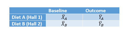 Although the mean weights per hall are the same at outcome as at baseline, some students have lost weight and some have gained weight, so the correlation between baseline and outcome is less than 1. However, the variances are the same at baseline and at outcome and, indeed, from one hall to another as indeed is the correlation. In further discussion I shall assume that we have the same number of students per hall.
Two statisticians (say John and Jane) now prepare to analyse the data. John uses a so-called change-score (the difference between weight at outcome and weight at baseline for every student). Once he has averaged the scores per hall, he will be calculating the difference
(YB – XB) – (YA– XA) = ( YB – YA) – (XB – XA ) = D – D = 0.
John thus concludes that there is no effect of diet on weight. Jane, on the other hand, proposes to use analysis of covariance. This is equivalent to ‘correcting’ each student’s weight at outcome by the within-halls regression of the weight at outcome on baseline. Since the variances at baseline and outcome are the same, this is equivalent to correcting the weights by the correlation coefficient, r. We can skip some of the algebra here but it turns out that Jane calculates
( YB – YA) – r(XB – XA ) = D – rD = (1 – r)D,
which is not equal to zero unless r = 1. However, that is not the case here and so a difference is observed. Jane, furthermore, finds that this is extremely significantly different from 0. Hence, Jane concludes that there is a difference between the diets. Who is right?

Figure 1. Baseline and outcome weights for the students in Hall A (red circles) and Hall B (blue squares). The black line is the line of equality along which John adjusts weights and the red and blue lines are those fitted by Jane in an analysis of covariance and used to adjust weights.
A graphical representation is given in Figure 1, where we can see that if we adjust along the line of equality there is no difference between the halls but if we adjust using the within groups regression there is.
The Book of Why points out that the initial weight X is a confounding variable here and not a mediator stating, ‘Therefore, the second statistician would be unambiguously correct here.’ (P216) My analysis, however, is slightly different. Basically, I consider that the first statistician is unambiguously wrong but that the second statistician is not unambiguously right. Jane may be right but this depends on assumptions that need to be made explicit. I shall now explain why.
As Holland and Rubin point out, a key to understanding the paradox is to try and think causally: is there a causal question and if so what does it imply? The way I usually try and understand these things is by imagining what I would do if it were a reasonable experiment, which, as we shall see, it is not and then consider what further adjustments are necessary.
Genstat® versus Lord’s paradox
So let us first of all assume that in order to understand the effects of diet, each of the two halls had been randomised to the diet. What would a reasonable analysis be? I shall start the investigation by considering outcomes only and see what John Nelder’s theory of the analysis of experiments(7, 8), as encoded in Genstat® would lead us to conclude. I shall then consider the role of the baseline values. I assume, just for illustration, that we have 100 students per hall and have created a data-set with exactly this situation: two halls, one diet per hall, 100 students per hall.
To analyse the structure, Genstat®, requires me to declare the block structure first. This is how the experimental material is organised before anything is done to it. Here we have students nested within halls. This is indicated as follows
BLOCKSTRUCTURE Hall/Student
Here “/” is the so-called nesting operator. Next, I have to inform the program of the treatment structure. This is quite simple in this case. There is only one treatment and that is Diet. So I write
TREATMENTSTRUCTURE Diet
Note that this difference between blocking and treatment structure is fundamental to John Nelder’s approach and, indeed, where not explicit, implicit in the whole approach of the Rothamsted school to designed experiments and thus to Genstat®. Without taking anything away from the achievements of the causal revolution outlined in The Book of Why it is interesting to note an analogy to the crucial difference between see (block structure) and do (treatment structure) in Pearl’s theory.
Next I need to inform Genstat® what the outcome variable is via an ANOVA statement, for example,
ANOVA Weight
but if I don’t, and just write
ANOVA
all that it will do is produce a so-called null analysis of variance as follows:
Analysis of variance
Source of variation d.f.
Hall stratum
Diet 1
Hall.Student stratum 198
Total 199
This immediately shows a problem. The problem is, in a sense obvious, and I am sure many a reader will consider that I have taken a sledgehammer to crack a nut but in my defence I can say, however obvious it is, it appears to have been rather overlooked in the discussion of Lord’s paradox. The problem is that, as any statistician can tell you, it is not enough to produce an estimate, you also have to produce an estimate of how uncertain the estimate is. Genstat® tells me here that this is impossible. The block structure defines two strata: the hall stratum and the student-within-hall stratum (here indicated by Hall.Student). There is only one degree of freedom in the first stratum but unfortunately the treatment appears in this stratum and competes for this single degree of freedom with what has to be used for error variation, namely the difference between halls. There is nothing that can be said using the data only about how precisely we have estimated the effect of diet and, if this is the case, the estimate is useless. The problem is that what we have is the structure of what in a clinical trials context would be called a cluster randomised trial with only two clusters.
What happens if I re-arrange my experiment to deal with this? Let us accept an implicit practical constraint that we cannot allocate students in the same hall to different diets but let us suppose that we can recruit more halls. Suppose that I could recruit 20 halls, ten for each diet with the same number of students studied in total, so that each hall provides ten students and, as before, I have 200 students. The Genstat® null ANOVA now looks like this.
Analysis of variance
Source of variation d.f.
Hall stratum
Diet Experiment 1 1
Residual 18
Hall.Student stratum 180
Total 199
We can see now, even more clearly, that it is the hall stratum that provides the residual variation with which we can estimate the precision of the treatment estimate and furthermore that whatever the contribution of studying students may be to making our experiment more precise, we cannot use the degrees of freedom within halls to estimating how precise it will be unless we can declare that the contribution to the overall variance of halls is zero. This is an important point to remember because it is now time we considered the baseline weight.
Suppose that we now stop to compare John’s and Jane’s estimates in terms of our improved experiment. Given that we have more information (if the variance between halls is important) we ought to expect to find that the values will differ less. First note that only the term ( YB – YA) can reflect the difference in diets and that this term is the same for both John and Jane’s estimate. Therefore, any convergence of John’s and Jane’s estimate is not because the term ( YB – YA) will estimate the causal effect of diet better, although it may very reasonably be expected to do so, since that virtue is reflected in both their approaches. Note also that diet can only affect this term, since the terms XB – XA involving occur before the dietary intervention.
No. The reason that we may expect some convergence is that although the correction term, involving the baselines is not the same for both statisticians, for both it is a multiple of the same difference. For John we have ( XB – XA) and for Jane we have r( XB – XA) and the difference between the two is (1 – r)( XB – XA) and this may be expected to get smaller as the number of halls increases. In fact, over all randomisations it is zero and if we keep the number of students per hall constant but increase the number of hall it approaches zero, so that in some sense we can regard both John and Jane as measuring the same effect marginally.
Now, it is certainly my point of view(9) that we should not be satisfied with such marginal arguments, although they should always be considered because they are calibrating. The consequence of this is that although marginal inferences do not trump conditional ones, if you get your marginal inference wrong you will almost certainly do the same with your conditional one. But suppose, we have a large number of halls but notice some particular difference at baseline in weights between the two groups of halls, be it large or be it small. What should we do about it? It turns out that if we can condition on this difference appropriately we will have an estimate that is a) independent of the observed difference and b) efficient (that is to say has a small variance). It is also known that a way to do this, that works, asymptotically at least, is analysis of covariance. So we should adjust the difference in weights at outcome using the differences in weights at baseline in an analysis of covariance. Doesn’t this get us back to Jane’s solution?
Not quite. The relevant difference we would observe is the relevant difference between the groups of halls. What Jane was proposing to do was to use the correlation within halls to correct a difference between. However, we have already seen that the Hall.Student stratum is not relevant for judging the variance of the outcomes. Can it automatically be right for judging the covariance? No. It might be an assumption one chooses to make but it will be a choice and it certainly cannot be said that this choice would be unambiguously right. If we just rely on the data, then Genstat® will have the baseline covariate entering in both strata, that is to say not only within halls but between.
Thus, my conclusion is that Jane’s analysis could be right if the within-hall variances and covariances are relevant to the variation across halls. They might be relevant but it is far from obvious that they must be and it therefore does not follow that Jane’s argument is unambiguously right.
Of course, what I described was what one would decide for an experiment. You may choose to disagree that such a supposedly randomised experiment could provide any guidance for something quasi-experimental such as Lord’s paradox. After all, we are not told that the diets were randomised to the halls. I am not so sure. I think that in this case, at least, the quasi-experimental set-up inherits the problems that the similar randomised experiment would show. I think that it is far from obvious that what Jane proposes to do is unambiguously right.
Whether you agree or disagree, I hope I have succeeded in showing you that statistical theory, and in particular careful examination of variation, a topic initiated by RA Fisher one hundred years ago(10) and for which he proposed the squared measure and gave it the name variance, goes beyond merely warning that correlation is not causation. Sometimes correlation isn’t even correlation.
(Associated slides are below.)
References
- Lord FM. A paradox in the interpretation of group comparisons. Psychological Bulletin. 1967;66:304-5.
- Senn SJ. Change from baseline and analysis of covariance revisited. Statistics in Medicine. 2006;25(24):4334–44.
- Pearl J, Mackenzie D. The Book of Why: Basic Books; 2018.
- Van Breukelen GJ. ANCOVA versus change from baseline had more power in randomized studies and more bias in nonrandomized studies. Journal of clinical epidemiology. 2006;59(9):920-5.
- Wainer H, Brown LM. Two statistical paradoxes in the interpretation of group differences: Illustrated with medical school admission and licensing data. American Statistician. 2004;58(2):117-23.
- Holland PW, Rubin DB. On Lord’s Paradox. In: Wainer H, Messick S, editors. Principals of Modern Psychological Measurement. Hillsdale, NJ: Lawrence Erlbaum Associates; 1983.
- Nelder JA. The analysis of randomised experiments with orthogonal block structure I. Block structure and the null analysis of variance. Proceedings of the Royal Society of London Series A. 1965;283:147-62.
- Nelder JA. The analysis of randomised experiments with orthogonal block structure II. Treatment structure and the general analysis of variance. Proceedings of the Royal Society of London Series A. 1965;283:163-78.
- Senn SJ. Seven myths of randomisation in clinical trials. Statistics in Medicine. 2013;32(9):1439-50.
- Fisher RA. The correlation between relatives on the supposition of Mendelian inheritance. Transactions of the Royal Society of Edinburgh. 1918;52:339-433.


")


Response to Stephen Senn post “Rothamsted Statistics meets
Lord’s Paradox,
by
Judea Pearl
Professor of Computer Science and Statistics
University of California Los Angeles
Summary
—————-
It is incorrect and overly defensive to interpret the Book
of Why as saying that “all that statisticians
ever did with causation is point out that correlation does
not mean causation.” What The Book observes is that,
lacking an adequate language, most statisticians prefer to terminate
causal conversations with “Additional assumptions are needed”
rather than state those assumptions formally and examine if
they are sufficient for answering research questions of interest.
Senn’s post substantiates these observations.
http://bayes.cs.ucla.edu/WHY/
Introduction, or which statistician is right?
—————-
Paradoxes are powerful tools for unveiling both
the working of the mind, and the paradigmatic
differences that set scientists apart. I was anxious therefore
to read how a prominent statistician, Stephen Senn,
would react to my analysis of Lord’s paradox as
described in The Book of Why (2018, with D. Mackenzie).
His reaction confirmed my expectations as well as
the critical observations that The Book of Why makes
about the role of causality in statistics.
Senn spends the bulk of his post on adjustments
in randomized trials, while his reaction to Lord’s paradox
which surfaces in nonrandomized setups, is summarized
in the following three conclusions:
——————–
1. the first statistician is unambiguously wrong
2. the second statistician is not unambiguously right.
3. depends on assumptions that need to be made explicit
Before analysing these conclusions, let me ask some
preliminary questions:
How do we know whether any of these three statements is in
fact true? Can we demonstrate that the second statistician (Jane)
may actually be wrong? In what language can we conduct the
demonstration? What are those “assumptions” that are
needed to prove Jane right? Can we articulate at least
one such assumption?
The Question of Language
——————————
My contention is that the traditional language of
statistical analysis, the one used throughout Senn’s
discussion, is helpless when it comes to answering
these questions.
Why? Because Lord asked a causal question: “To determine the
effect of diet,” while the language of classical statistics
is a language of associations, sitting
on rung-1 of the Ladder of Causation (Chapter 1).
The two do not mix. In other words, unless a statistician is willing
to acquire new notation for causal concepts
that cannot be assessed from raw data
(eg. “effect of”, “potential outcome”, “confounding”)
he/she will be unable to evaluate, or even
verify which statistician is right and which is wrong.
Interestingly, and most revealing, although Senn’s
admits to be influenced by Holland and Rubin’s
realization that Lord’s paradox requires causal thinking,
none of this causal thinking enters any of the
mathematical expressions that are used in his post. All
the formal expressions are part of the pre-Rubin language
of expectations, correlations, and conditionalization,
that is, relationships that can be estimated from the
data. Rubin’s “potential outcome” notation does not appear
in Senn’s analysis, despite the fact that with this notation
one can articulate the untestable assumptions that would
tell us which statistician is right.
Why hasn’t Senn used Rubin’s notation in a problem that
obviously requires causal thinking? The answer reflects on
the practice of a whole century of statistics.
Senn states it thus: “very little of what I have ever
done as a statistician has had anything to do with
correlation but rather a lot with causation.”
Indeed, most statisticians are driven by causal questions,
some even spend their entire career struggling with
such questions. Unfortunately, only few have recognized
that the textbook language of statistics is incapable
of handling such questions, and even those who adopted
Rubin’s potential outcome notation would fail to
use it correctly on problems like Lord’s paradox,
which involve confounding and mediation.
[Such problems, as explain in Chapter 4 of The Book of Why,
are practically unsolvable without the use of
graphical models and, graphs, by acts of neglect,
are still not part of standard statistical education.]
The Role of Untestable Assumptions
———————————
I now address Senn’s third statement:
“3. depends on assumptions that need to be made explicit”
which is re-stated in slide 45 as:
“Additional untestable assumptions would be needed.”
This statement is true about any causal conclusion
drawn from every observational
study. It applies therefore to John as well as to Jane.
Thus, if the second statistician is not unambiguously right.
the first statistician cannot be unambiguously wrong.
If we exclude “untested assumptions” then no statistician
can be unambiguously right or unambiguously wrong. On the
other hand, if we
accept “untested assumptions” they can tell us
unambiguously which statistician is right and which is wrong.
In either case, one of Senn’s conclusions must be wrong.
Surely additional untestable assumptions would be needed
to resolve Lord’s dilemma; it is after all a causal dilemma.
The question before us is: What do we do when we are given
a set of untestable assumptions, say that the initial weight is the only
variable that can conceivably affect both the final weight
and the choice of diet. Can we determine which statistician
is right contingent on this assumption?
Specifically, if we accept the assumptions encoded in the
graph, can we determine unambiguously which statistician
would be right and which will be wrong?
This is not the kind of question statisticians are trained
to answer, I admit. Dealing with untestable assumptions,
especially when encoded in graphical form, is
not part of statistical vocabulary. What The Book of Why
claims is that, lacking an adequate language,
most statisticians prefer to terminate
causal conversations with “Additional assumptions are needed”
rather than state those assumptions and examine if they are
sufficient for answering their research questions.
The Book tells us how to do that formally and painlessly.
What assumptions are needed?
Looking over Senn’s 47 slides, a viewer might get the impression
that (see slide 45):
“* A lesson is that we need to consider the probability
distribution of an inference, e.g., at least the variance.”
This impression would be misleading. No amount of
distributional information could replace the
assumptions needed to resolve Lord’s
paradox. Any statistician who hopes that some statistical
assumptions would be sufficient would be waiting
in false hopes from here to eternity.
The New Game in Town: Causal Inference
——————————–
The new game in town is: we are given the pair:
{data + assumptions}, what can we conclude from
their combination.
In his final slide (46) Senn concludes that:
“It is an open question for me whether the causal calculus in
its current form is adequate to deal with complex data-sets.”
Fortunately, the causal calculus in its current form possesses a
property called “completeness”, which essentially states that
no one cannot do better. This means that if we find
a problem that the causal calculus cannot solve, we can
rest assured that NO method can solve it — the problem is
simply UNSOLVABLE.
I should also note that the causal calculus is reducible
to a polynomial time algorithm for estimating causal relations.
This should be kept in mind when we consider
“complex data-sets”
Finally, readers who are interested in a more
complete analysis of Lord’s paradox and its associated “Sure
Thing Principle” can find accessible accounts here:
https://ucla.in/2JeJs1Q and here: https://ucla.in/2NTbnrS
Judea Pearl
First let me reassure Judea Pearl that none of my remarks are in anyway intended to be disparaging. I have been an admirer ever since I read his 2000 book and in my own book of 2003, Dicing with Death, I explain that he deserves the credit for having provided a complete and correct solution to Simpson’s paradox. The solution is obviously right in retrospect but it still had to wait half a century for Pearl to present it (or even longer if we regard Yule as the originator) and I regard it as important. In my lecture at Edinburgh I took along my copy of The Book of Why, which circulated among the audience while I gave my lecture. I hope that I persuaded at least some of those present that it was a book that they needed to read.
However, if Pearl looks at my presentation he will see that I do not use the mathematical expressions except either to claim that the they are misleading or that other arguments are needed to judge how they behave. At no point does the conventional algebra drive what I have to say. I use other arguments altogether in particular paying close attention to what can actually be changed by any cause (baselines can’t), how any expressions we use will behave as we go to a case where the answer is obvious, and how uncertainty about what we see must be judged.
I also, don’t see in his reply to my comments that he has done John Nelder’s approach to designed experiments justice. This does make a crucial causal distinction between blocking factors and treatment factors. In fact, I think that Pearl and I could probably agree on much if he appreciated that Genstat, which incorporates Nelder’s ideas is different in this respect from any other package. As far as I am aware you won’t find it in R, SAS, SPSS or STATA. In other words Genstat is different because it reflects a view on designed experiments that is causal. Nelder’s approach is limited to certain types of investigation and does not cover observational studies and It clearly does not have the scope and ambition of Pearl’s causal calculus but it is very powerful for complex designed experiments. The reason I spent so much time on randomised experiments was that I was claiming that an analysis that was wrong in a randomised experiment could also be so in a close non-randomised analogue and therefore the randomised set up might be worth considering.
So here is my suggestion. Perhaps Pearl could show us how the causal calculus addresses these four cases where, in each case the effect (causal question) of diet on weight is being studied .
1) Two diets have been randomised in a designed experiment to two halls of 100 students each. (One diet per hall.) Weight at the end of the academic year is measured but it was forgotten to do so at the beginning.
2) As in 1) above but we now have 20 halls, 10 halls per diet but with 10 students in each hall
3) As in 2) above but we now have baseline measurements of weight as well as measurements of weight at the end
4) As in 1) above so now we are back to two halls only with 100 students each but we do have baseline measurements. (This is basically a randomised example of the Wainer and Brown set-up)
To this, by the way, an interesting 5th case can be added. This is as case 3 but records have been lost and all that we have (in addition to which hall used which diet) are the mean weights per student per hall at baseline and outcome.
In my opinion, applying Nelder’s approach to these four cases, which is what I did in my lecture, reveals that unless you wish to make assumptions about between and within-hall variance and covariance components that are actually quite strong and have been rather overlooked in the past, simple analysis of covariance will not give you the right answer.
After reading this post, you would almost think that Stephen Senn is a fan of GenStat
Well spotted, Zad. I am indeed a fan of Genstat. Its approach to analysis of designed experiments is quite different from any other package as far as I am aware. I believe that Brian Cullis and Alison Smith are working on getting John Nelder’s approach implemented in an R package. Until they do, all of you non-Genstat users must continue to inhabit the outer darkness in which light cannot be shed on the difference between blocking and treatment factors.
Stephen Senn seems to be enchanted by Nedler’s approach to complex experimental designs. I can’t share this enchantment because I fail to see its relevance to Lord’s paradox as described by Lord in 1967 and which requires an observational study to surface.
I totally agree however with the following statement of Senn:
“Nelder’s approach is limited to certain types of investigation and
does not cover observational studies and It clearly does not have
the scope and ambition of Pearl’s causal calculus but it is very
powerful for complex designed experiments. The reason I spent
so much time on randomised experiments was that I was claiming
that an analysis that was wrong in a randomised experiment could
also be so in a close non-randomised analogue
and therefore the randomised set up might be worth considering.”
It might be worth considering if the paradox was framed in terms of the fine details of the distributions created by diet-1 vs. diet-2. But the paradox appears already in the expected value of the weight gain.
There is no need to go down to distributional details, or to finite-sample analysis, where
statistics proper can perform miracles. Tha causal calculus was developed to handle
problems where statistics proper hangs helpless, if not parralized — resolving causal paradoxes that
offends our sense of right and wrong.
Judea Pearl
Professor
UCLA Computer Science Department
3531 Boelter Hall
Los Angeles, CA 90095-1596
310.825.3243
judea@cs.ucla.edu
I fear that I have not succeeded in getting my point across. Let me attempt a brief clarification. I believe that Professor Pearl and I agree that the correct approach to analyse the weight data is to correct the weights at outcome by conditioning on the initial weights in an analysis of covariance. This appears to be one of the two approaches offered by Lord himself.
However, what the Rothamsted school approach shows is that in the context “analysis of covariance” is itself ambiguous because there are two covariances not one. One is the covariance within halls between baseline and final weights and the other is the corresponding covariance between halls. Lord proposes the former as a possible correction (it is one of the approach he considers) but Nelder’s approach suggest the latter. I agree with Nelder. I assume that Pearl does not.
Of course, given the paucity of data (there are only two halls), the Nelder approach cannot be implemented. The fact that this is so, however, does not make an approach (such as correcting using the within-hall covariance) correct just because it can be implemented. It might be a reasonable approximation, it might not, but it cannot be unambiguously right.
John is right, but for the wrong reasons.
There are multiple problems with many of the arguments presented by John and Jane.
First of all, the two Hall groups differ considerably in their weight distributions.
The Figure 1 graph says the red circles are the Hall A residents, and the blue squares are the Hall B residents. (Confusingly, the Hall A resident glyphs in the slides of John’s analysis are blue circles and the Hall B resident glyphs are red squares. So we’ll go with the shapes rather than the colours.)
The Hall A residents show a lower average weight in September than the Hall B residents. So the two groups are not equal. This is of course why the diets should have been randomly assigned to hall residents rather than confounding diet with hall.
So of course any analysis procedure should properly consider this group difference in assessing weight changes. Thus Jane should of course not attribute the difference in intercept values to diet, shame on Jane. A diet difference would show as a difference in slope values, or a difference in intercept values beyond (1-r)D. Jane should expect that under the null hypothesis of no difference in weight gain patterns, the slopes of the two regression lines will not differ, and the intercept difference will be near (1-r)D. That’s just how regression lines work for bivariate normal data with the same correlation, same variance, but different means.
John should have fit three principle component lines, one for the whole group and one for each hall. In this case the lines would all lie on top of one another. If a weight gain differential existed between the halls, the three principle component lines would not show equal slope and/or intercept values.
And of course even if the differences in slopes or intercept values varied from that expected under a no weight gain differential hypothesis, the difference could not be attributed to diet without considering what else was going on in those halls. If Hall A was a sorority and Hall B was a fraternity we would expect such a weight distribution differential given that women tend to be smaller on average than men. But naturally in that scenario behavioural differences could explain a weight gain differential as readily as a diet-induced difference, which randomization of diet would have handled nicely as well.
I have to disagree. The solution given in the Book of Why is correct in expectation provided that the between halls regression is the same as the within halls regression. The standard error would still be wrong unless there is no component of variation attributable to hall.
As a practical note, of course if the diet is delivered by the hall’s canteen individual assignment of diet is not possible. The quasi-experiment actually employed is analogous to what is called cluster randomised in the clinical trials world.
Just a historical note: I believe Nelder did in fact use potential outcomes in his papers on general balance, though not by that name.
(Nelder’s model also worked under the assumption of “unit-treatment additivity”, i.e. no effect heterogeneity.)
Dear leonnnn. Thanks you may be right about potential outcomes and Nelder. I need to go back to the papers. I think that if one uses a Fisherian approach then “unit-treatment additivity” is guaranteed under the null but not necessarily when the null hypothesis is false.
Pingback: S. Senn: “Error point: The importance of knowing how much you don’t know” (guest post) | Error Statistics Philosophy