

.
Stephen Senn
Consultant Statistician
Edinburgh, Scotland
Testing Times
Screening for attention
There has been much comment on Twitter and other social media about testing for coronavirus and the relationship between a test being positive and the person tested having been infected. Some primitive form of Bayesian reasoning is often used to justify concern that an apparent positive may actually be falsely so, with specificity and sensitivity taking the roles of likelihoods and prevalence that of a prior distribution. This way of looking at testing dates back at least to a paper of 1959 by Ledley and Lusted[1]. However, as others[2, 3] have pointed out, there is a trap for the unwary in this, in that it is implicitly assumed that specificity and sensitivity are constant values unaffected by prevalence and it is far from obvious that this should be the case.
In the age of COVID-19 this is a highly suitable subject for a blog. However, I am a highly unsuitable person to blog about it, since what I know about screening programmes could be written on the back of a postage stamp and the matter is very delicate. So, I shall duck the challenge but instead write about something that bears more than a superficial similarity to it, namely, testing for model adequacy prior to carrying out a test of a hypothesis of primary interest. It is an issue that arises in particular in cross-over trials, where there may be concerns that carry-over has taken place. Here, I may or may not be an expert, that is for others to judge, but I can’t claim that I think I am unqualified to write about it, since I once wrote a book on the subject[4, 5]. So this blog will be about testing model assumptions taking the particular example of cross-over trials.
Presuming to assume
The simplest of all cross-over trials, the so-called AB/BA cross-over is one in which two treatments A and B are compare by randomising patients to one of two sequences: either A followed by B (labelled AB) or B followed by A (labelled BA). Each patient is thus studied in two periods, receiving one of the two treatments in each. There may be a so-called wash-out period between them but whether or not a wash-out is employed, the assumption will be made that by the time the effect of a treatment comes to be measured in period two, the effect of any treatment given in period one has disappeared. If such a residual effect, referred to as a carry-over, existed it would bias the treatment effect since, for example, the result in period two of the AB sequence would not only reflect the effect of giving B but the previous effect of having given A.
Everyone is agreed that if the effect of carry-over can be assumed negligible, an efficient estimate of the difference between the effect of B and A can be made by allowing each patient to act as his or her own control. One way of doing this is to calculate a difference for each patient of the period two values minus the period one values. I shall refer to these as the period differences. If the effect of treatment B is the same as that of treatment A, then these period differences will not be expected to differ systematically from one sequence to another. However, if (say) the effect of B was greater that that of A (and higher values were better), then in the AB sequence a positive difference would be added to the period differences and in the BA sequence that difference would be subtracted from the period differences. We should thus expect the means of the period differences for the two sequences to differ. So one way of testing the null hypothesis of no treatment effect is to carry out a two-sample t-test comparing the period differences between one sequence an another. Equivalently from the point of view of testing, but more convenient from the point of view of estimation, is to work with the semi period differences, that is to say the period difference divided by two. I shall refer to the associated estimate as CROS and the t-statistic for this test as CROSt, since they are what the crossover trial was designed to produce.
Unfortunately, however, these period differences could also reflect carry-over and if this occurs it would bias the estimate of the treatment effect. The usual effect will be to bias it towards the null and so there may be a loss of power. Is there a remedy? One possibility is to discard the second period values. After all, the first period values cannot be contaminated by carry-over. On the other hand single period values is what we have in any parallel group trial. So all we need to do is regard the first period values as coming from a parallel group trial. Patients in the AB sequence yield values under A and patients in the BA sequence yield values under B so a comparison of the first period values, again using a two-sample t-test, is a test of the null hypothesis of no difference between treatments. I shall refer to this estimate as the PAR statistic and the corresponding t-statistic as PARt.
Note that the PAR statistic is expected to be a second best to the CROS statistic. Not only are half the values discarded but since we can no longer use each patient as his or her own control, the relevant variance is a sum of between and within-patient variances unlike for CROS, which only reflects within-patient variation. Nevertheless, PAR may be expected to be unbiased in circumstances where CROS will be and since all applied statistics is a bias-variance trade-off it seems conceivable that there are circumstances under which PAR would be preferable.
Carry-over carry on
However, there is a problem. How shall we know that carry-over has occurred? It turns out that there is a t-test for this too. First, what we construct are means over the two periods for each patient. In each sequence such means must reflect the effect of both treatments, since each patient receives each treatment and they must also reflect the effect of both periods, since each patient will be treated in each period. However, in the AB sequence the total (and hence the mean) will also reflect the effect of any carryover from A in the second period whereas in the BA sequence the total (and hence the mean) will reflect the carry-over of B. Thus, if the two carry-overs differ, which is what matters, these sequence means will differ and therefore the t-test of the totals comparing the two sequences is a valid test of zero differential carry-over. I shall refer to the estimate as SEQ and the corresponding t-statistic as SEQt.
The rule of three
These three tests were then formally incorporated in a testing strategy known as the two-stage procedure[6]as follows. First a test for carry-over was performed using SEQt. Since the test was a between-patient test and therefore of low power, a nominal type I error rate of 10% was generally used. If SEQt was not significant, the statistician proceeded to use CROSt to test the principle hypothesis of interest, namely that of the equality of the two treatments. If however, SEQt was significant, which might be taken as an indication of carry-over, the fallback test PARt was used instead to test equality of the treatments.
The procedure is illustrated in Figure 1.
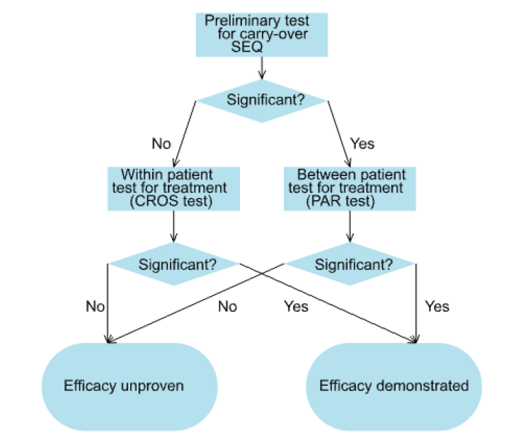
Figure 1. The two-stage procedure.
Chimeric catastrophe
Of course, to the extent that the three tests are used as prescribed, they can be combined in a single algorithm. In fact in the pharmaceutical company that I joined in 1987, the programming group had written a SAS® macro to do exactly that. You just needed to point the macro at your data and it would calculate SEQ, come to a conclusion, choose either CROS or PAR as appropriate and give you your P-value.
I hated the procedure as soon as I saw it and never used it. I argued that it was an abuse of testing to assume that just because SEQ was not significant that therefore no carry-over has occurred. One had to rely on other arguments to justify ignoring carry-over. It was only on hearing a colleague lecture on an example where the test for carry-over had proved significant and, much to his surprise, given its low power, the first period test had also proved significant, that I suddenly realised that SEQ and PAR were highly correlated and therefore this was only to be expected. In consequence, the procedure would not maintain the Type I error rate. Only a few days later a manuscript from Statistics in Medicine arrived on my desk for review. The paper by Peter Freeman[7] overturned everything everyone believed on testing for carry-over. In bolting these tests together, statisticians had created a chimeric monster. Far from helping to solve the problem of carry-over the two-stage procedure had made it worse.
‘How can screening for something be a problem?’, an applied statistician might ask but in asking that they would be completely forgetting the advice they would give a physician who wanted to know the same thing. The process as a whole of screening plus remedial action needed to be studied and statisticians had failed to do so. Peter Freeman completely changed that. He did what statisticians should have done and looked at how the procedure as whole behaved. In the years since I have simply asked statisticians who wish to give an opinion on cross-over trials what they think of Freeman’s paper[7]. It has become a litmus paper for me. Their answer tells me everything I need to know.
Correlation is not causation but it can cause trouble
So what is the problem? The problem is illustrated by Figure 2. This shows a simulation from a null case. There is no difference between the treatments and no carry-over. The correlation between periods one and two has been set to 0.7. One thousand trials in 24 patients (12 for each sequence) have been simulated. The figure plots CROSt(blue circles) and PARt (red diamonds) on the Y axis against SEQt on the X axis. The vertical lines show the critical boundaries for SEQt at the 10% level and the horizontal lines show the critical boundaries for CROSt and PARt at the 5% level. Filled circles or diamonds indicate significant results of CROSt and PARt and open circles or diamonds indicate non-significant values.
It is immediately noticeable that CROSt and SEQt are uncorrelated. This is hardly surprising, since given equal variances CROS and SEQ are orthogonal by construction. On the other hand PARt and SEQt are very strongly correlated. This ought not to be surprising. PAR uses the first period means. SEQ also uses the first period with the same sign. Even if the second period means were uncorrelated with the first the two statistics would be correlated, since the same information is used. However, in practice the second period means will be correlated and thus a strong correlation can result. In this example the empirical correlation is 0.92.
The consequence is that if SEQt is significant PARt is likely to be so. This can be seen from the scatter plot where there are far more filled diamonds in the regions to the left of the lower critical value or to the right of the higher critical values for SEQt than in the region in between. In this simulation of 1000 trials, 99 values of SEQt are significant at the 10% level 50 values of CROSt and 53 values of PARt are significant at the 5% level. These figures are close to the expected values. However, 91 values are significant using the two-stage procedure. Of course, this is just a simulation. However, for the theory[8] see http://www.senns.demon.co.uk/ROEL.pdf .
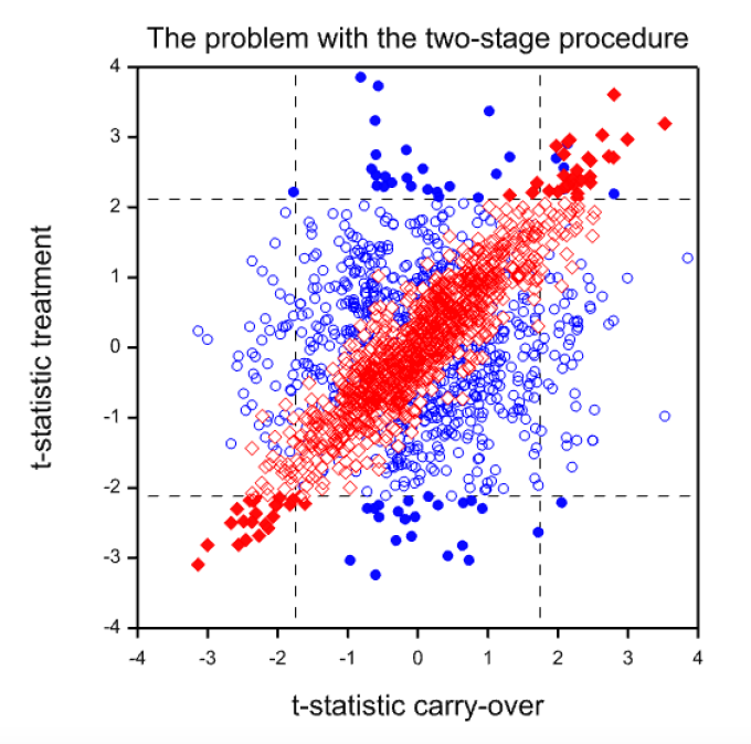
Figure 2. Scatterplot of t-statistics (CROSt) for the within-patient test (blue circles) or the t-statistics (PARt) for the between-patient test (red diamonds) against the value of the t-statistic (SEQt) for the carry-over test. Filled values are ‘significant’ at the 5% level.
In fact, this inflation really underestimates the problem with the two-stage procedure. Either the extra complication is irrelevant (we end up using CROSt) or the conditional type-I error rate is massively inflated. In this example, of the 99 cases where SEQt is significant, 48 of the values of PARt are significant. A nominal 5% significance rate has become nearly a 50% conditional one!
What are the lessons?
The first lesson is despite what your medical statistics textbook might tell you, you should never use the two-stage procedure. It is completely unacceptable.
Should you test for carry-over at all? That’s a bit more tricky. In principle more evidence is always better than less. The practical problem is that there is no advice that I can offer you as to what to do next on ‘finding’ carry-over except to drop the nominal target significance level. (See The AB/BA cross-over: how to perform the two-stage analysis if you can’t be persuaded that you shouldn’t[8], but note the warning in the title.)
Should you avoid using cross-over trials? No. they can be very useful on occasion. Their use needs to be grounded in biology and pharmacology. Statistical manipulation is not the cure for carry-over.
Are there more general lessons? Probably. The two-stage analysis is the worst case I know of but there may be others where testing assumptions is dangerous. Remember, a decision to behave as if something is true, is not the same as knowing it is true. Also, beware of recogiseable subsets. There are deep waters here.
References
- Ledley, R.S. and L.B. Lusted, Reasoning foundations of medical diagnosis; symbolic logic, probability, and value theory aid our understanding of how physicians reason. Science, 1959. 130(3366): p. 9-21.
- Dawid, A.P., Properties of Diagnostic Data Distributions. Biometrics, 1976. 32: p. 647-658.
- Guggenmoos-Holzmann, I. and H.C. van Houwelingen, The (in)validity of sensitivity and specificity.Statistics in Medicine, 2000. 19(13): p. 1783-92.
- Senn, S.J., Cross-over Trials in Clinical Research. First ed. Statistics in Practice, ed. V. Barnett. 1993, Chichester: John Wiley. 257.
- Senn, S.J., Cross-over Trials in Clinical Research. Second ed. 2002, Chichester: Wiley.
- Hills, M. and P. Armitage, The two-period cross-over clinical trial. British Journal of Clinical Pharmacology, 1979. 8: p. 7-20.
- Freeman, P., The performance of the two-stage analysis of two-treatment, two-period cross-over trials.Statistics in Medicine, 1989. 8: p. 1421-1432.
- Senn, S.J., The AB/BA cross-over: how to perform the two-stage analysis if you can’t be persuaded that you shouldn’t., in Liber Amicorum Roel van Strik, B. Hansen and M. de Ridder, Editors. 1996, Erasmus University: Rotterdam. p. 93-100.


")


I’m very grateful to Stephen Senn for his guest post on “Testing Times”. The times we are living in are indeed testing people’s ability to cope. But Senn’s post isn’t about that—at least not directly. It deals with an issue that arises in cross-over medical trials, although he tantalizingly hints that the problem he discusses has at least a “superficial similarity” to the problem of diagnostic screening for Covid-19 when “it is implicitly assumed that specificity and sensitivity are constant values unaffected by prevalence”. His hesitancy to come out and reveal the similarity he has in mind, claiming he lacks sufficient expertise (on medical screening), just tantalizes this reader into guessing at the intended analogy. I hope that we can draw him out in the discussion.
In any event, one of the lessons Senn draws is that “testing for model adequacy prior to carrying out a test of a hypothesis of primary interest” can in some cases be “dangerous”. Of course it would be best to ground assumptions about how long the effect of a treatment lasts on biology and pharmacology, as he suggests. Perhaps the lesson is that flawed statistical tests of assumptions, and especially their flawed uses in subsequent statistical tests, can be dangerous because they can wreck, rather than help to ensure, the error probabilities of the primary test. But I definitely lack the expertise to speculate about the particular case.
This is very nice and a very good example for problems with combined procedures in which a test is decided based on a preliminary test for the validity of model assumptions. I wasn’t aware of this and will need to incorporate it here:
M. Iqbal Shamsudheen, Christian Hennig (2020), Should we test the model assumptions before running a model-based test? https://arxiv.org/abs/1908.02218
By the way, Stephen, if you have any more ideas on what may be missing in that preprint, please tell me!
I can’t resist quoting the last two sentences of Peter Freeman’s paper
“Once they are allowed, a perfectly satisfactory analysis of the two-period, two-treatment crossover trial becomes available, that of Grieve.9 In my opinion this is the only satisfactory analysis and, in the light of the results in this paper, the two-stage analysis is so unsatisfactory as to be ruled out of future use.”
The paper of mine that Peter Freeman was referring had appeared in Biometrics in 1985. While these two sentences are extremely supportive of the Bayesian approach developed in that paper, I now agree with Stephen that there is a major flaw with the approach which I then espoused.
The flaw is fundamental to most approaches to analysing crossover designs. What is wrong is that most approaches fail to acknowledge that an additive model in which the treatment and carryover effect are handled independently ignores the practical issue that it is extremely unlikely that the carryover is larger in magnitude than the treatment effect.
In our 1998 joint paper, while commenting on my Bayesian approach, Stephen wrote “I am prepared to stick my neck out and say that when we finally get a Bayesian method of analysing crossover trials that models the dependency between carryover and treatment ( and I am prepared to make the Bayesian statement that AG is the person most likely to produce it), the simple CROS analysis will be shown to provide reasonable results in practice, even where carryover is appreciable, unless the sample size of the trial is extremely large.” Unfortunately I haven’t as yet.
Andy and Stephen:
Can either of you explain how the recognition that the carryover is larger than the treatment effect wrecks the 2-stage approach? When I first read Senn on this issue several years ago, I recall getting to the point of understanding the problem he was raising with the 2-stage approach (which might differ from your point), but I couldn’t recover my understanding in time for this post. I’d appreciate insights on any aspects to recover what I understood, or thought I did, about this problem. Thanks so much.
I think that there are two separate issues. The first is that although testing for carry-over would be reasonable if it were known it would be enormous if ever it occurred, in practice the test turns out to be not so much a way of identifying carry-over but a way of identifying bad randomisations. However, if a bad randomisation occurs, the last thing you want to do is use a between-subject test. The within-subject test is immune to bad randomisations but the between-subject test is extremely vulnerable to it. This is what the simulation shows.
The second point is the one that Andy refers to. If one wishes to cure this by employing a Bayesian approach, then in addition to the correlation between the statistics PAR and SEQ to which my blog refers, there is the issue of correlation of parameters. Over all classes of treatments and diseases it seems much more reasonable to suppose that large carry-over effects are rare if treatment effects are modest. Handling this by finding suitable joint priors is not so easy. A similar situation arises in connection with random effects meta-analysis and an amateurish effect of mine to handle it can be found here: https://www.onlinelibrary.wiley.com/doi/abs/10.1002/sim.2639
Stephen:
Can you explain why “testing for carry-over …turns out to be not so much a way of identifying carry-over but a way of identifying bad randomisations”? Thank you.
Suppose that, just by bad luck, having randomisaed, there is an excess of patients in one group who will do badly, whatever treatment they are given. In a parallel group trial you cannot recognise this directly using the outcome values since the the two groups differ by treatment given. Hence you won’t know whether randomisation or treatment is responsible. The probability calculations of the significance test are there to help you decide. You can recognise a bad randomisation indirectly, however, by examining covariates and, of course, a superior analysis is to condition on prognostic covariates, whether or not they are imbalanced.
However, for a cross-over trial, the two groups do not differ by treatment given; they only differ by the order in which they were given. Hence, if you calulate the mean over both periods for patients, these means do not reflect differences in the treatment given. There are only two things that they could reflect 1) an effect of the order in which treatments are given (carry-over is a plausible explanation) and 2) a bad randomisation.
Thus, if you could dismiss carry-over as an explanation you would have a perfect way of identifying bad randomisations but, ironically, provided that your subsequent treatment test was based on within-patient differences, it would not matter. On the other hand it does matter if you use first period values alone. But this is what PAR does. So it turns out, that far from keeping you safe, pre-testing would lure you into danger.
Stephen:
I realize you’ve written a whole book on carry-over trials, which I don’t have, but I take the main justification for blogs to be to provide an opportunity to try to engage at some level, to learn something valuable and new, even if it remains a half-baked understanding.
So for now, this is just on the basis of your blogpost. I number my queries.
The two-staged testing, as I understand it (and I do not claim to have any but the most fragile grasp) will look at the totals from the AB and BA sequences, and if these differ statistically significantly, the second period is thrown away and only the first period results are compared in the PAR test. Is that right?
“However, in the AB sequence the total (and hence the mean) will also reflect the effect of any carryover from A in the second period whereas in the BA sequence the total (and hence the mean) will reflect the carry-over of B. Thus, if the two carry-overs differ, which is what matters, these sequence means will differ and therefore the t-test of the totals comparing the two sequences is a valid test of zero differential carry-over.”
(2) The subjects in the AB sequence differ from those in the BA sequence. But to detect carryover, shouldn’t each subject be treated in each order (AB and BA)? Maybe this is infeasible, but I’m not sure why.
(3) You don’t say if B is placebo in your blog or another treatment. But in any event, why would the second period just be thrown out? Couldn’t the carry-over effect be estimated?
(4) You write that “I suddenly realised that SEQ and PAR were highly correlated and therefore this [finding statistical significance at the PAR stage] was only to be expected. In consequence, the procedure would not maintain the Type I error rate.” The conditional Type I error rate is much higher. Is this what happens? When the “no carryover null hypothesis” is erroneously rejected, it increases the probability that the “no treatment effect null hypothesis” is erroneously rejected because you have an experimental group that just happens to be higher/lower than the other, quite apart from the treatment.
It does seem very odd to have supposed it was OK to assume the result from the first stage (the test of the “no carryover” assumption) could just be used in running the second test, without considering the overall error probability (associated with the primary inference). OK, that’s my attempt to grasp this. Doubtless this reveals the huge gap in my understanding here, but since I’m fortunate enough to have your guest contribution, I will stick my neck out and see if I can’t get a little clearer.
Deborah:
1)Yes you are right about the way that the two-stage procedure works. It is as described in the flow diagram in the blog.
2) Testing each subject in each order would lead to an ABBA/BAAB design. These double the amount of time the patient has to spend in the trial and are rarely attempted. They are also covered in my book but that is another complicated story I don’t want to go into here.
3) Estimating the carry-over effect is what comparing the mean per patient over the two periods between the two sequences does. Adjusting for this leads to just using the first period data so acheives nothing different.
4) Yes. The correlation between the two statistics is the cause of the problem. In fact although unconditionally CROS and PAR have different variances, conditionally on SEQ they have the same variance. In fact given any two you can tell what the third is. It is also the case that although PAR is uncinditionally unbiased it is not conditionally unbiased. This is why I like this problem so much. Thinking about it carefully leads one to realise that bias and variance are just two sides of the same coin. Once one has learned the lesson one then starts to look for the problem everywhere.
Yes I think it was odd to make that mistake but it’s potentially a wider problem. For example, what is the Type I error rate of the two stage procedure under Normaility? 1) Test for Normality using Shapiro-Wilks 2) a) If Normality accepted use t-test b)If Normality rejected use Wilcoxon rank sum test. I don’t know. Christian Henning might know.
> what is the Type I error rate of the two stage procedure under Normaility? 1) Test for Normality using Shapiro-Wilks 2) a) If Normality accepted use t-test b)If Normality rejected use Wilcoxon rank sum test.
Or for a given design and set of assumptions one could do a simulation (as in my comment below).
It is nice when experts can and are willing to provide an answer, but simulation is a general approach that with persistence allows one to answer almost any error rate question…
Keith O’Rourke
@Stephen & Mayo: The earlier linked paper reviews (among other things) literature where this was simulated. It has a general review on “combined procedures”, i.e., procedures in which a model assumption is tested first, and conditionally on the result of the test of the model assumption, a procedure is chosen that requires this model assumption, or another one that doesn’t.
https://arxiv.org/abs/1908.02218
I actually believe that this is pretty important and central, also for your philosophy of frequentist testing, because these studies investigate to what extent model assumption testing may harm in some situations (and your philosophy seems to rely on the idea that model assumptions can be tested in order to make sure they are valid). The literature that investigated this is overall surprisingly skeptical about model assumption tests and many of these papers advise against it. In our paper we argue that this is partly correct in the sense that many specific procedures of this kind don’t work very well, however we are generally more positive because we believe that a general setup from which data could be generated (which we treat with a little theory only in that paper, although we have simulations that will be published probably separately) can give more positive outcomes for such procedures *if the involved tests are chosen correctly*. In practice unfortunately it depends on a number of details whether it is good or not, some of which are hard to assess. Particularly whether and which such a procedure is worthwhile depends a lot on the “violating” true model in case the model assumptions are violated. (In case of testing for normality for deciding whether a nonparametric test or a t-test should be used, confusingly there exist two papers that both advise *against* normality testing, however one of them recommends a rank test always, the other one recommends a t-test always, because they used different non-normal distributions in their simulations. The user may therefore still want to have a decision rule, i.e., test, for distinguishing in which of these situations we are.
Stephen:
Just a word on my point #2: I wasn’t imagining a change in the entire design, but rather to use the data already collected to check any change from the order.
I also don’t see that an estimation is achieved by the test (my point #3). Maybe there was a carryover but it turns out to be trivial-no grounds to throw out half the data.
Well, never mind, thank you for the post, which encouraged me to look into this.
Thanks, not sure I recall the Freeman paper but certainly do recall yours.
Now the first time I had to analyze a cross-over trial I by habit simulated the full process so was able to discern the benefit/risks of various approaches. I had gotten into the habit of simulating anything I did not think I clearly understood after Larry Wasserman organized a seminar when we were graduate students (1980s), on the Monte Hall problem. I just simulated that game which requires all assumptions be fully clarified. Then you discern what repeatedly happens. So I never understood the fuss – if Monte has to choose between two doors to open and does so randomly 50/50 – then the is no information from which opened. If he has a bias there is information but in any case its always better to switch.
OK went on a bit about that silly game, but point the point is over 40 years later still difficult to convince people what’s important is what repeatedly happens in the full data acquisition and analysis processing pipeline (in either Frequentist or Bayesian terms) and simulation is a “no brainer” way to discern that. Today to almost any level of accuracy given enough persistence.
Keith O’Rourke
Diagnostic test assessment has more in common with RCTs than screening
I became rather excited when you started referring to diagnostic testing but because I have no practical experience and therefore a proper understanding of designing RCTs, I wouldn’t get involved in any discussion on cross-over trials. However, during the Covid-19 crisis, many felt quite free to discuss diagnostic tests even though it appears that they had no practical experience of the diagnostic process and its detailed nature. They based their opinion on sensitivities and specificities intended only for assessing screening and did not consider plotting distributions of the screening results in those with and without target outcomes but dichotomised them (I suspect to your displeasure) according to long-standing dogma and thus throwing away information. Diagnosis has far more in common with RCTs than over-simplified screening models
The main problem is that until we can draw up sensible diagnostic criteria for all those and only those in whom a working diagnosis can be justified, we cannot assess the ability of other findings to predict that diagnosis. Such diagnostic criteria have not been agreed yet for Covid-19, which is why people are going around in circles talking about speculative sensitivities, specificities, false positive and false negative rates based mostly on personal opinion, theories and various aspects of probability theory. Dispiritingly, those who licence tests also base their assessments on sensitivity and specificity with little emphasis on evidence for the underlying diagnostic criteria. The latter’s main purpose is not to allow sensitivities and specificities to be calculated for those who wish to do so but to make preliminary predictions about disease outcomes with or without interventions.
A working diagnosis simply tells us that a number of treatments or advice based on prognosis might be helpful. However, for each possible treatment, we still have to identify the treatment indication criteria based on RCT entry criteria and the outcome of that RCT before a sufficiently accurate prediction of what will happen with and without that treatment can be accurate enough to make sensible decisions. Because of their preliminary nature, the criteria for a diagnosis need not be high powered; they can be many and varied (i.e. there are usually multiple ‘sufficient’ criteria). They are simply guidelines as to when a making a provisional working diagnosis is sensible and when a group of treatments or prognoses should be considered and further information looked for.
Experienced diagnosticians regard the diagnostic process as common sense. With an emerging illness like Covid-19, the important thing is to identify the predictions that need to be made about the possible treatments, other interventions and advice (e.g. isolating those with the suspected diagnoses and their contacts). Once these required predictions and their indications have been identified, it is possible to design diagnostic and treatment indication criteria. Most doctors dealing with Covid-19 in public health, primary care and hospitals will have already arrived at these diagnostic criteria individually and intuitively; they will be using them informally during differential diagnosis and treatment selection. Hopefully they will be supported soon by evidence from suitable studies, especially further RCTs.
An important device for diagnosticians is a list of diagnoses with prior probabilities conditional on a symptom, sign or test result and the various sufficient criteria for acting on the working diagnoses in this list as in the Oxford Handbook of Clinical Diagnosis. This reasoning process can be modelled by a theorem derived from the extended version of Bayes rule that uses differential odds or differential likelihood ratios between pairs of diagnoses in that list (not between a diagnosis and its ‘absence’ based on sensitivities and false positive rates or specificities). It exploits mathematical (as opposed to statistical) independence in the same way as simultaneous equations. It also addresses the proportion of patients not covered by the diagnoses in the list. This allows abductive reasoning to take place where the probability of a diagnosis ‘or something else’ can be estimated. The same model can be applied to scientific hypothetico-deductive reasoning, to severe testing of diagnostic test reliability and showing that P-hacking etc. are hopefully absent when interpreting P values.
Diabetic nephropathy as a possible outcome of type 2 diabetes mellitus provides an example of basing diagnoses on RCTs. It has been established by RCTs that an ACE inhibitor or angiotensin receptor blocker can reduce the frequency of nephropathy and more so in high risk patients. Doctors understand intuitively that the severity of a disease affects the benefit from treatment. For example, the higher the albumin excretion rate (AER), the higher the risk and the greater the risk reduction with treatment (modelled by odds ratios). The severity of the diabetes as measured by the HbA1c is another predictor of nephropathy but the effect of an ACEI or ARB on risk reduction is not predicted well by the level of the HbA1c. However, the latter is a good predictor for the effect of treatments that reduce blood glucose (e.g. insulin). These predictive qualities depend on an intelligent application of biochemistry, physiology and clinical trial design. The degree of severity of the predictor would then become an important diagnostic criterion.
An established or final diagnosis is usually the diagnosis still being considered when a decision is made not to change its associated treatments or advice for the time being or for good. This does not necessarily mean that it is correct. The patient should not be labelled with a diagnosis if there is danger of more harm than good (e.g. from stigma in the absence of helpful treatment). It is sensible therefore to have a large number of sufficient criteria for working diagnoses in order that as many patients as possible are considered for its interventions, but not to label patients unless they have a high probability of benefit as evidenced by an RCT and there has been improvement on one of its interventions as well (not necessarily ‘due’ to the intervention as some would improve on placebo). This established or final diagnosis is analogous to an established theory that is not to be tested for the time being.