Stephen Senn
Consultant Statistician
Edinburgh, Scotland

Alpha and Omega (or maybe just Beta)

Well actually, not from A to Z but from AZ. That is to say, the trial I shall consider is the placebo- controlled trial of the Oxford University vaccine for COVID-19 currently being run by AstraZeneca (AZ) under protocol AZD1222 – D8110C00001 and which I considered in a previous blog, Heard Immunity. A summary of the design  features is given in Table 1. The purpose of this blog is to look a little deeper at features of the trial and the way I am going to do so is with the help of geometric representations of the sample space, that is to say the possible results the trial could produce. However, the reader is warned that I am only an amateur in all this. The true professionals are the statisticians at AZ who, together with their life science colleagues in AZ and Oxford, designed the trial.

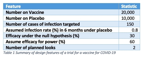
Whereas in an October 20 post (on PHASTAR) I considered the sequential nature of the trial, here I am going to ignore that feature and only look at the trial as if it had a single look. Note that the trial employs a two to one randomisation, twice as many subjects being given vaccine as placebo

However, first I shall draw attention to one interesting feature. Like the two other trials that I also previously considered (one by BioNTech and Pfizer and the other by Moderna) the null hypothesis that is being tested is not that the vaccine has no efficacy but that its efficacy does not exceed 30%. Vaccine Efficacy (VE) is defined as

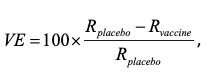
Where R_placebo & R_vaccine are the ‘true’  rates of infection under placebo and vaccine respectively

Obviously, if the vaccine were completely ineffective, the value of VE would be 0. Presumably the judgement is that a vaccine will be of no practical use unless it has an efficacy of 30%. Perhaps a lower value than this could not really help to control the epidemic. The trial is designed to show that this is the case. In what follows, you can take it as read that the probability of the trial failing because the efficacy is equal to some value that is less than 30% (such as 27%, say) is even greater than if the value is exactly 30%. Therefore, it becomes of interest to consider the way the trial will behave if the value is exactly 30%.

Figuring it out

Figure 1 gives a representation of what might happen in terms of cases of infected subjects in both arms of the trial based on its design. It’s a complicated diagram and I shall take some time to explain it. For the moment I invite the reader to ignore the concentric circles and the shading. I shall get to those in due course.

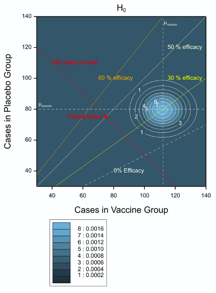Figure 1 Possible and expected outcomes for the trial plotted in the two dimensional space of vaccine and placebo cases of infection. The contour plot applies when the null hypothesis is true.

The X axis gives the number of cases  in the vaccine group and the Y axis the number of cases under Placebo. It is important to bear in mind that twice as many subjects are being treated with vaccine as with placebo. The line of equality of infection rates is given by the dashed white diagonal line  towards the bottom right hand side of the pot and labelled ‘0% efficacy’. This joins (for example) the points (80,40) and (140, 70) corresponding to twice as many cases under vaccine as placebo and reflecting the 2:1 allocation ratio. Other diagonal lines correspond to 30%, 50% and 60% VE respectively.

The trial is deigned to stop once 150 cases of infection have occurred. This boundary is represented by the diagonal solid red line descending from the upper left (30 cases in the vaccine group and 120 cases in the placebo group) towards the bottom right (120 cases in the vaccine group and 30 cases in the placebo group). Thus, we know in advance, that the combination of results we shall see must lie on this line.

Note that the diagram is slightly misleading, since where the space concerned refers to number of cases, it is neither continuous in X nor continuous in Y. The only possible values are those given by the whole numbers, W, that is to say the integers plus zero. However, the same is not true for expected numbers and this is a common difference between parameters and random variables in statistics. For example, if we have a Poisson random variable with a given mean, the only possible values of the random variable are the whole numbers 0,1,2… but the mean can be any positive real number.

Ripples in the pond

Figure 2 is the same diagram as Figure 1 as regards every feature except that which I invited the reader to ignore. The concentric circles are contour plots that represent features of the trial that are suitable for planning. In order to decide how many subjects to recruit, the scientists at AZ and Oxford had to decide what infection rate was likely. They chose an infection rate of 0.8% per 6 months under placebo. This in turn implies that of 10,000 subjects treated with placebo, we might expect 80 to get COVID. On the other hand, a vaccine efficacy of 30% would imply an infection rate of 0.56% since 

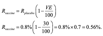
For 20,000 subjects treated with vaccine we would expect (0.56/100)20,000 = 112 of them to be infected with COVID and if the vaccine efficacy were 60%, the value assumed for the power calculation, then the expected infection rate would be 0.32% and we would expect 64 of the subjects to be infected.

Since the infection rates are small, a Poisson distribution is a possible simple model for the probability of seeing certain combinations of infections. This is what the contour plots illustrate. For both cases, the expected number of cases under placebo is assumed to be 80 and this is illustrated by a dashed horizontal white line. However, the lower infection rate under H₁ has the effect of shifting the contour plots to the left. Thus, in Figure 1 the dashed vertical line indicating the expected numbers in the vaccine arm is at 112 and in Figure 2 it is at 64. Nothing else changes between the figures.

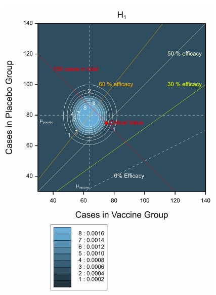
Figure 2 Possible and expected outcomes for the trial plotted in the two dimensional space of vaccine and placebo cases of infection. The contour plot applies when the value under the alternative hypothesis assumed for power calculations  is true.

Test bed

How should we carry out a significance test? One way of doing so is to condition on the total number of infected cases. The issue of whether to condition or not is a notorious controversy ins statistics, Here the total of 150 is fixed but I think that there is a good argument for doing so whether or not it is fixed. Such conditioning in this case leads to a binomial distribution describing the number of cases of infection observed out of the 150 that are in the vaccine group. Ignoring any covariates, therefore, a simple analysis, is to compare the proportion of cases we see to the proportion we would expect to see under the null hypothesis. This proportion is given by 112/(112+80)=0.583. (Note a subtle but important point here. The total number of cases expected is 192 but we know the trial will stop at 150. That is irrelevant. It is the expected proportion that matters here.)

By trial and error or by some other means we can now discover that the probability of 75 or fewer cases given vaccine out of 150 in total when the probability is 0.583 is 0.024.The AZ protocol requires a two-sided P-value less than or equal to 4.9%, which is to say 0.0245 one sided, assuming the usual doubling rule, so this is just low enough.  On the other hand, the probability of 76 or fewer cases under vaccine is 0.035 and thus too high. This establishes the point X=75, Y=75 as a critical value of the test. This is shown by the small red circle labelled ‘critical value’ on both figures. It just so happens that this lies along the 50% efficacy line. Thus observed 50% efficacy will be (just) enough to reject the hypothesis that the true efficacy is 30% or lower.

Reading the tea-leaves 

There are many other interesting features of this trial I could discuss, in particular what alternative analyses might be tried (the protocol refers to a ‘modified Poisson regression approach’ due to Zou, 2004) but I shall just consider one other issue here. That is that in theory when the trial stops might give some indication as to vaccine efficacy, a point that might be of interest to avid third party trial-watchers. If you look at Figure 3, which combines Figure 1 and Figure 2, you will note that the expected number of cases under H­₀, if the values used for planning are correct,  is at least (when vaccine efficacy is 30%) 80+112=192. For zero efficacy the figure is 80+160=240. However, the trial will stop once 150 cases of infection have been observed. Thus, under H₀, the trial is expected to stop before all 30,000 subjects have had six months of follow-up.

On the other hand, for an efficacy of 60% given in Figure 3 the value is 80+64 =144 and so slightly less then the figure required. Thus, under H₁, the trial might not be big enough. Taken together, these figures imply that other things being equal, the earlier the trial stops the more likely the result is to be negative and the longer it continues, the more likely it is to be positive.

Of course, this raises the issue as to whether one can judge what is early and what is late. To make some guesses as to background rates of infection is inevitable when planning a trial. One would be foolish to rely on them when interpreting it.

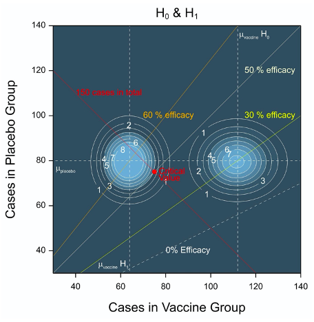
Figure 3 Combination of Figures 1 and 2 showing contour plots for the joint density for the number of cases when the vaccine efficacy is 30% (H₀) and the value under H₁ of 60% used for planning.

Reference

Zou G. A modified poisson regression approach to prospective studies with binary data. Am J Epidemiol. 2004;159(7):702-6.

POSTSCRIPT: Needlepoint

Pressing news

Extract of a press-release from Pfizer, 9 November 2020:

“I am happy to share with you that Pfizer and our collaborator, BioNTech, announced positive efficacy results from our Phase 3, late-stage study of our potential COVID-19 vaccine. The vaccine candidate was found to be more than 90% effective in preventing COVID-19 in participants without evidence of prior SARS-CoV-2 infection in the first interim efficacy analysis.” Albert Bourla (Chairman and CEO, Pfizer.)

Naturally, this had Twitter agog and calculations were soon produced to try and reconstruct the basis on which the claim was being made: how many cases of COVID-19 infection under vaccine had there been seen in order to be able to make this claim? In the end these amateur calculations don’t matter. It’s what Pfizer calculates and what the regulators decide about the calculation that matters. I note by the by that a fair proportion of Twitter seemed to think that journal publication and peer review is essential. I don’t share this point of view, which I tend to think of as “quaint”. It’s the regulator’s view I am interested in but we shall have to wait for that.

Nevertheless, calculation can be fun and if I don’t think so, I am in the wrong profession. So here goes. However, first I should acknowledge that Jen Rogers’s interesting blog on the subject has been very useful in preparing this note.

The back of the envelope

To do the calculation properly, this is what one would have to know

Need to know	Discussion
Disposition of Subjects	Randomisation was one to one but strictly speaking we want to know the exact achieved proportions. BusinessWire describe a total of “43,538 participants to date, 38,955 of whom have received a second dose of the vaccine candidate as of November 8, 2020”.
Number of cases of infection	According to BusinessWire 94 were seen.
Method of analysis	Pfizer claims in the protocol a Bayesian analysis will be used. I shall not attempt this but use a very simple frequentist one conditioning on totals infected.
Aim of claim	Is the point estimate the basis of the claim or is the lower bound of some confidence interval the basis?
Level of confidence to be used	Pfizer planned to look five times but it seems that the first look was abandoned. The reported look is the 2nd but at a number of cases that is slightly greater (94) than the number originally planned for the 3rd (92). I shall assume that the confidence level for look three of an O’Brien-Fleming boundary is appropriate.
Missingness	A simple analysis would assume no missing data or at least that any missing data are missing completely at random.
Other matters	Two doses are required. Were there any cases arising between the two doses and if so, what was done with them?

 

If I condition on the total number of infected cases, and assume equal numbers of subjects on each arm, then by varying the number of cases in the vaccine group and subtracting them from the total of 94 to get those on the control group arm, I can calculate the vaccine efficacy. This has been done in the figure below.

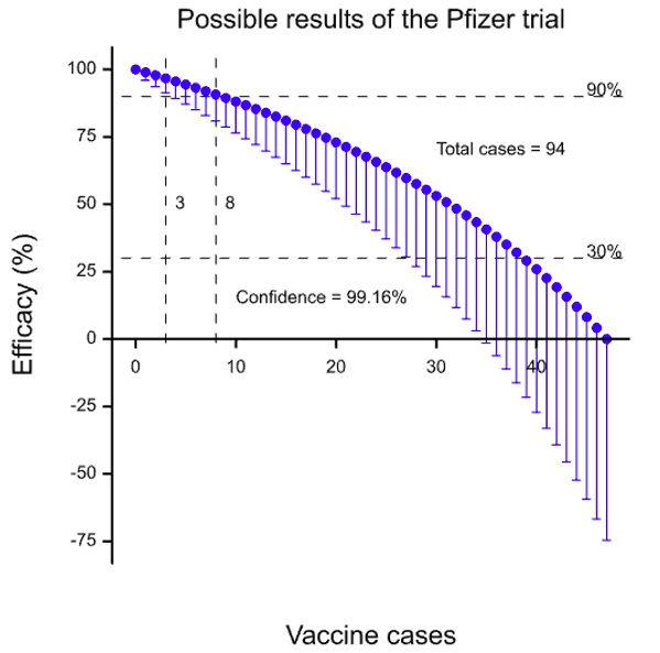
The solid blue circles are the estimate of the vaccine efficacy. The ‘whiskers’ below indicate a confidence limit of 99.16% which (I think) is the level appropriate for the third look in an O’Brien-Fleming scheme for an overall type I error rate of 5%. Horizontal lines have been drawn at 30% efficacy (the value used in the protocol for the null hypothesis) and 90% efficacy (the claimed effect in the press release). Three cases on the vaccine arm would give a vaccine efficacy at about 91.3% for the lower confidence interval whereas four gives a value of 89.2%. Eight cases would give a point estimate of 90.7%. So depending on what exactly the claim of “more than 90% effective” might mean (and a whole host of other assumptions) we could argue that between three and eight cases of infection were seen.

Safety second

Of course safety is often described as being first in terms of priorities but it usually takes longer to see the results that are necessary to judge it than to see those for efficacy. According to BusinessWire “Pfizer and BioNTech are continuing to accumulate safety data and currently estimate that a median of two months of safety data following the second (and final) dose of the vaccine candidate – the amount of safety data specified by the FDA in its guidance for potential Emergency Use Authorization – will be available by the third week of November.”

The world awaits the results with interest.

A Dec. 2, 2020 update by Senn

https://www.linkedin.com/pulse/needlework-guesswork-stephen-senn/

Reference

556. C. O’Brien and T. R. Fleming (1979) A multiple testing procedure for clinical trials. Biometrics, 549-556.