

.
Deirdre McCloskey’s comment leads me to try to give a “no headache” treatment of some key points about the power of a statistical test. (Trigger warning: formal stat people may dislike the informality of my exercise.)
We all know that for a given test, as the probability of a type 1 error goes down the probability of a type 2 error goes up (and power goes down).
And as the probability of a type 2 error goes down (and power goes up), the probability of a type 1 error goes up. Leaving everything else the same. There’s a trade-off between the two error probabilities.(No free lunch.) No headache powder called for.
So if someone said, as the power increases, the probability of a type 1 error decreases, they’d be saying: As the type 2 error decreases, the probability of a type 1 error decreases! That’s the opposite of a trade-off. So you’d know automatically they’d made a mistake or were defining things in a way that differs from standard NP statistical tests.
Before turning to my little exercise, I note that power is defined in terms of a test’s cut-off for rejecting the null, whereas a severity assessment always considers the actual value observed (attained power). Here I’m just trying to clarify regular old power, as defined in a N-P test.
^^^^^^^^^^^^^^^^^^^^^^^^^^^^^^^^^^^^^^^^^^^^^^^
Let’s use a familiar oversimple example to fix the trade-off in our minds so that it cannot be dislodged. Our old friend, test T+ : We’re testing the mean of a Normal distribution with n iid samples, and (for simplicity) known, fixed σ:
H0: µ ≤ 0 against H1: µ > 0
Let σ = 2, n = 25, so (σ/ √n) = .4. To avoid those annoying X-bars, I will use M for the sample mean. I will abbreviate (σ/ √n) as σx .
- Test T+ is a rule: reject H0 iff M > m*
- Power of a test T+ is computed in relation to values of µ > 0.
- The power of T+ against alternative µ =µ1 = Pr(T+ rejects H0 ;µ = µ1) = Pr(M > m*; µ = µ1)
We may abbreviate this as : POW(T+,α, µ = µ1)
(1) First test (test 1): T+ with α = .02: To avoid headaches even further, let test 1 use the 2σx cut-off, α = .02 (approx), even though 1.96 is a more familiar cut-off for α = .025.
The cut-off for rejecting: m*.02 = 0+ 2(2)/√25 = .8. Test T+ rejects H0 at the .02 level if M > 2(.4) = .8. The cut-off m*.02 = .8.
Cool Fact #1: The power of test T+ to detect an alternative that exceeds the cut-off m* by 1σx =.84.[i]
In test 1, the alternative μ1 that exceeds the cut-off m* by 1σx = m* + 1(.4) = .8 + .4 = 1.2.
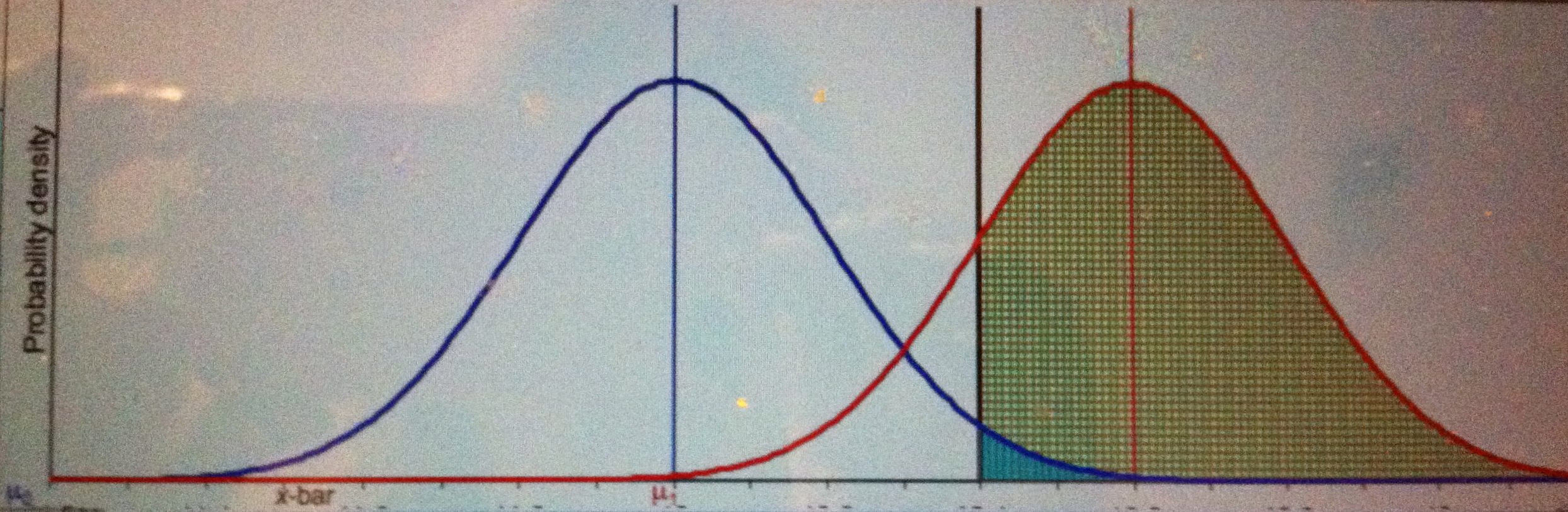
So test T+ rejects the null with probability .84 under the assumption that µ = 1.2:
POW(T+,α = .02, µ = 1.2) = .84.
The red curve below is the alternative µ = 1.2, and the green area is the power of the test under µ = 1.2.
EXERCISE ONE
(2) Second test (test 2): Now consider we are instructed to decrease the type 1 error probability α to .001, but it’s impossible to get more samples. This requires the cut-off to be further away from 0 than when α = .02: the cut-off must be 3σx greater than 0 rather than only 2σx so now the cut-off is:
m*.001 = 0+ 3(2)/√25 = 3(.4) = 1.2.
We decrease α (the type 1 error probability) from .02 to .001 by moving the hurdle (m*) over to the right by 1 σx unit. Against what value of µ does this test have .84 power? We know from our cool fact:
The power of test T+ to detect an alternative that exceeds the cut-off m* by 1σx =.84. So we can easily fill in the ? in the following:
POW(T+,α = .001, µ = ?) = .84.
To replace the ?, set µ = m* + 1σx
µ = 1.2. + (.4) = 1.6. So, POW(T+,α = .001, µ = 1.6) = .84.
- Decreasing the type 1 error (of the test 1) by moving the hurdle over to the right by 1 σx unit (making the hurdle for rejection higher) results in the alternative against which we have .84 power also moving over to the right by 1 σx .
- So we see the trade-off very neatly, at least in one direction.
- Of course the alternative against which the test has .84 power is the alternative against which the type 2 error probability is 1 – .84 = .16.
QUESTION: What’s the POW(T+, µ = 1.2) now that we’ve changed the cut-off to m*.001 ?
Pr(M ≥ m*; µ = 1.2) = Pr(Z ≥ (1.2- 1.2)/.4) = Pr(Z ≥ 0) = .5.
Notice here the cut-off m* happens to equal to the value of µ for which we are computing the power. We get a general result in test T+: this is always .5.
Cool Fact #2: POW(T+, µ = m*) = .5. This is a very useful benchmark that saves many headaches. Notice:
- Test 1: The power to detect (µ = m*.02 = .8) = .5
- Test 2: The power to detect (µ = m*.001= 1.2) = .5.
Since test 2 makes it harder to reject the null than test 1, it’s cut-off m* is bigger, so the value against which it has power .5 is bigger. That means test 2 is less powerful than test 1. That’s because we reduced the probability of a type 1 error.
A power of .5 is rather lousy, but notice the value of µ that test 1 is this lousy at detecting is smaller than the value of µ that test 2 is this lousy at detecting. Again, test 2 has less power than test 1. Compare the power of the two tests for a fixed alternative µ = 1.2:
- Test 1: POW(µ = 1.2) = .84
- Test 2: POW(µ = 1.2) = .5.
By lowering the type 1 error probability (from .02 to .001), we’ve lowered the power to detect µ = 1.2. Raising the threshold for rejecting the null (higher hurdle) => lowering the type 1 error probability=>lowering the power of the test against any alternative.[ii] ——————————————-
I’m not saying anything in this post about interpreting tests (which I’ve done elsewhere on this blog), nor the desire for high power, nor the problems with some ways power has been misused, or any such thing. I’m just getting at the trade-off in relation to test hurdles.
EXERCISE TWO is next


")


I almost called this “no headache powder power” which is kind of a tongue twister.
This is a good way to look at it. If alpha is moved to .16, so the cut-off m* is only one standard unit (.4) greater than 0, then m* = .4, and by this niftily trick, the alternative against which my new test has .84 power is m* + .4 = .8! Yes? In relation to test 1, this new test has moved m* one standard (.4) unit to the left, and as a result the alternative against which the new test has .84 power is one unit to the left of 1.2. Given the test 1 had power of .84 against 1.2.
Yes, exercise two will consider how changing power results in changes to alpha.
Yeah, well, maybe. But you are focused laser-like on explaining power—the Lord’s work, surely—-yet do not in this communication mention the Greater Work of that same Lord. It is: getting practitioners to realize that translating into (frequentist) probabilities (and assuming contrary to fact that the main scientific problem is sampling error) and proceeding is not a sensible way of making scientific decisions unless (1.) you have no prior information at all (e.g. that the fellow offering to play dice with you is, or is not, a notorious cheat) and (2.) you or anyone else do not care at all how the test comes out, that is, you have no non-quadratic, non-symmetric loss function (Savage’s utility function) about over- or under-estimating some effect (e.g. you are testing an old lady’s ability to distinguished first-milk tea from first-tea in the cup of milky tea, not, say testing a powerful new drug that cures hepatitis C).
Ziliak and I point out that the two conditions for legitimacy for significance testing are rare (and of course they routinely ignore power, too, a point that would apply even to Fisher’s disastrously misleading example of the tea testing) .
Do you agree? If so, you should say so, right? It’s you responsibility as a statistician to set people right when they are using statistics in such an obviously idiotic way, yes? High priority, true? Higher even that getting them exactly right on the logic and maths of power, n’est ce pas? If you agree, please say so, in print.
Deirdre:
I’m not sure what the “maybe” is.
1. Admittedly, one is forced to spend more time than one would choose on simple significance tests because so much criticism and confusion surrounds them. The strictly formal significance test is a small part in an overall account of statistical inference which, as I see it, includes experimental design and data generation,collecting, modeling, drawing inferences from data. My own interpretation of tests always is in terms of discrepancies well or poorly warranted–never just reject at such and such levels. This is true for estimation as well.
The most noteworthy problems with reported significance levels in the daily handwringing may be separated into two (although they could well be combined) are: (a) the computed p-vaue is illicit and doesn’t report on the actual error probing capacities of tests (due to violated assumptions, cherry picking, selection effects, and assorted bias es) and (b) the statistical inference is divorced from the intended or claimed inference.
(They are combined into one by placing (b) under violated assumptions and biases.)
2. The idea that statistical inference of a frequentist variety includes no background information is absurd. I’ve discussed this at great length on this blog.
Click to access Article_Cox_Mayo.pdf
https://errorstatistics.com/2013/07/23/background-knowledge-not-to-quantify-but-to-avoid-being-misled-by-subjective-beliefs-2/
The background we need consists of known information about fallibilities, trickery and deceits regarding the type of inquiry in question. (They bring in magicians for ESP studies; we need to build a similar but much more general background repertoire to detect shams, chump effects, and to hold “trust us” experts accountable–at least those of us unwilling to give up data and evidence as a basis for claims)
3. I take the error statistical logic to apply at all levels of inquiry, formal, quasi-formal and informal. That is the point of introducing the general notion of severity and severe probes (of mistaken interpretations of data.)
This may be the reason you are having trouble grasping the missionary zeal I bring to concepts like power: it’s because the same logic follows in properly criticizing tests. But you will (and do) criticize tests incorrectly by incorrectly grasping such notions as power. Getting the concepts straight in the formal realm is akin to recognizing the formal validity of, say, disjunctive syllogism, and the invalidity of affirming the consequent knowing that in real-life arguments, they may enter informally.
4. If you get the formal reasoning wrong then, no matter how much you dress up your statistical inference or modelling, it’s still going to be mere window dressing: an object that looks science-y, but is actually fallacious and even the opposite of what you think you’re getting (as with power).
Adding our various “loss functions” to such a mess (as you claim to espouse, but maybe don’t really) only further disguises whatever small role your data might have played: why bother collecting it? Just report whatever is most prudential and best serves one’s interests or social negotiations (as the radical postmodernists hold). Evidence will then have no role in adjudicating disputes, it’s just a matter of whose got more clout. That’s a notion of power that is inimical to science, and to holding anybody accountable to evidence.
5. Finally, I’m a philosopher of science and statistics, not a statistician.
Pingback: “Only those samples which fit the model best in cross validation were included” (whistleblower) “I suspect that we likely disagree with what constitutes validation” (Potti and Nevins) | Error Statistics Philosophy