In defense of statistical recipes, but with enriched ingredients (scientist sees squirrel)

This bothers me, because we can’t do inference in science without statistics*. Why are students so unreceptive to something so important? In unguarded moments, I’ve blamed it on the students themselves for having decided, a priori and in a self-fulfilling prophecy, that statistics is math, and they can’t do math. I’ve blamed it on high-school math teachers for making math dull. I’ve blamed it on high-school guidance counselors for telling students that if they don’t like math, they should become biology majors. I’ve blamed it on parents for allowing their kids to dislike math. I’ve even blamed it on the boogie**.

All these parties (except the boogie) are guilty. But I’ve come to understand that my list left out the most guilty party of all: us. By “us” I mean university faculty members who teach statistics – whether they’re in Departments of Mathematics, Departments of Statistics, or (gasp) Departments of Biology. We make statistics needlessly difficult for our students, and I don’t understand why.

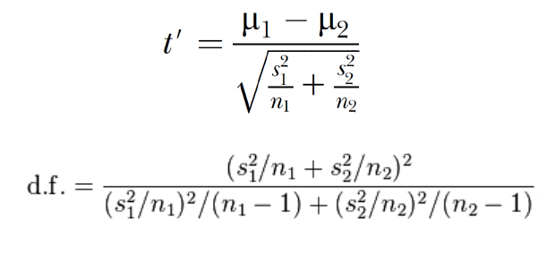
The problem is captured in the image above – the formulas needed to calculate Welch’s t-test. They’re arithmetically a bit complicated, and they’re used in one particular situation: comparing two means when sample sizes and variances are unequal. If you want to compare three means, you need a different set of formulas; if you want to test for a non-zero slope, you need another set again; if you want to compare success rates in two binary trials, another set still; and so on. And each set of formulas works only given the correctness of its own particular set of assumptions about the data.

Given this, can we blame students for thinking statistics is complicated? No, we can’t; but we can blame ourselves for letting them think that it is. They think so because we consistently underemphasize the single most important thing about statistics: that this complication is an illusion. In fact, every significance test works exactly the same way.

Every significance test works exactly the same way. We should teach this first, teach it often, and teach it loudly; but we don’t. Instead, we make a huge mistake: we whiz by it and begin teaching test after test, bombarding students with derivations of test statistics and distributions and paying more attention to differences among tests than to their crucial, underlying identity. No wonder students resent statistics.

What do I mean by “every significance test works exactly the same way”? All (NHST) statistical tests respond to one problem with two simple steps.

 The problem:

• We see apparent pattern, but we aren’t sure if we should believe it’s real, because our data are noisy.

 The two steps:

• Step 1. Measure the strength of pattern in our data.
• Step 2. Ask ourselves, is this pattern strong enough to be believed?

Teaching the problem motivates the use of statistics in the first place (many math-taught courses, and nearly all biology-taught ones, do a good job of this). Teaching the two steps gives students the tools to test any hypothesis – understanding that it’s just a matter of choosing the right arithmetic for their particular data. This is where we seem to fall down.

Step 1, of course, is the test statistic. Our job is to find (or invent) a number that measures the strength of any given pattern. It’s not surprising that the details of computing such a number depend on the pattern we want to measure (difference in two means, slope of a line, whatever). But those details always involve the three things that we intuitively understand to be part of a pattern’s “strength” (illustrated below): the raw size of the apparent effect (in Welch’s t, the difference in the two sample means); the amount of noise in the data (in Welch’s t, the two sample standard deviations), and the amount of data in hand (in Welch’s t, the two sample sizes). You can see by inspection that these behave in the Welch’s formulas just the way they should: t gets bigger if the means are farther apart, the samples are less noisy, and/or the sample sizes are larger. All the rest is uninteresting arithmetical detail.

Step 2 is the P-value. We have to obtain a P-value corresponding to our test statistic, which means knowing whether assumptions are met (so we can use a lookup table) or not (so we should use randomization or switch to a different test***). Every test uses a different table – but all the tables work the same way, so the differences are again just arithmetic. Interpreting the P-value once we have it is a snap, because it doesn’t matter what arithmetic we did along the way: the P-value for any test is the probability of a pattern as strong as ours (or stronger), in the absence of any true underlying effect. If this is low, we’d rather believe that our pattern arose from real biology than believe it arose from a staggering coincidence (Deborah Mayo explains the philosophy behind this here, or see her excellent blog).

Of course, there are lots of details in the differences among tests. These matter, but they matter in a second-order way: until we understand the underlying identity of how every test works, there’s no point worrying about the differences. And even then, the differences are not things we need to remember; they’re things we need to know to look up when needed. That’s why if I know how to do one statistical test – any one statistical test – I know how to do all of them.

Does this mean I’m advocating teaching “cookbook” statistics? Yes, but only if we use the metaphor carefully and not pejoratively. A cookbook is of little use to someone who knows nothing at all about cooking; but if you know a handful of basic principles, a cookbook guides you through thousands of cooking situations, for different ingredients and different goals. All cooks own cookbooks; few memorize them.

So if we’re teaching statistics all wrong, here’s how to do it right: organize everything around the underlying identity. Start with it, spend lots of time on it, and illustrate it with one test (any test) worked through with detailed attention not to the computations, but to how that test takes us through the two steps. Don’t try to cover the “8 tests every undergraduate should know”; there’s no such list. Offer a statistical problem: some real data and a pattern, and ask the students how they might design a test to address that problem. There won’t be one right way, and even if there was, it would be less important than the exercise of thinking through the steps of the underlying identity.

You can read the rest of his blogpost here.

When I was a graduate teaching assistant in statistics at the Wharton School, the students used to call the class “Sadistics”. It was for that class that I first created “statistical recipes”, which helped them a lot, and I’ve used them in teaching philosophy of statistics– enriched with philosophical ingredients. I agree with Heard on the importance of stressing the overall logic of statistical inference. Enriched “recipes” that explain the goals and underlying (testing) rationale of basic methods like significance tests are much more valuable than running computer programs. I’m strongly in favor of churning out results by hand to get at the patterns of reasoning.

It’s important, however, to treat reported P-values as “nominal” and not “actual” until they pass an audit. Results based on cherry-picking, multiple testing, optional stopping, fishing, barn-hunting, and a host of other biasing selection effects, readily produce impressive-looking P-values that are spurious. Violated statistical assumptions should also be part of auditing P-values, as with other error probabilities. It’s actually an asset of P-values, not a liability, that they are provably altered by biasing selection effects. The danger is with methods that do not directly pick up on such problems, or even declare they are irrelevant to evidence. (See this msc kvetch among my rejected posts.) 

Simple significance tests (generally with directional departures) have important roles, but something closer to Neyman-Pearson tests can avoid classic fallacies of rejection (as well as fallacies of negative results)––even though I favor a non-behavioristic interpretation. What is often called “a null hypothesis significance test (NHST)” in certain fields has little relation to Fisherian significance tests. If NHST permits going from a single small P-value to a genuine effect, it is illicit; and if it permits going directly to a substantive research claim it is doubly illicit! (It might be better to drop an acronym associated with so illicit an animal.)

Instead of recognizing and avoiding this well-known fallacy, many “reformers” forfeit statistical inferences altogether, often in favor of mere comparative assessments of plausibility. By giving lumps of prior probability to null hypotheses (usually of 0 effect), a Bayes Factor may be thought to show no evidence against, and even evidence for, a point null hypothesis, but in truth it only shows it scores higher relative to a particular chosen alternative (and often, relative as well to a chosen prior).[1] Among several untoward consequences, (a) this enshrines the illicit move from a statistical effect to a research hypothesis, and (b) it fails to identify methodological flaws with the studies. The way to genuinely debunk results is by identifying methodological flaws and demonstrating failures to replicate. It is fascinating to observe that the same fields that declare “it is too easy to obtain small P-values!” are the same ones that find it exceedingly difficult to obtain small P-values in preregistered replication studies! (I call this “The Paradox of Replication”.)

One remark on Heard’s note (*) that he will “refrain from snorting derisively at claims that we don’t need inferential statistics at all”. Please don’t.[2] When editors declare P-values “invalid” because they do not give posterior probabilities, set out with “test bans”, and “don’t ask don’t tell” policies, the worst thing is to refrain from calling them out.[3] A blogpost on the ban is here.

—

[1] In this spirit, it is argued that in order to block Bem’s inferences to ESP, we should appeal to its implausibility, and thus give a high prior to the null. (See Schimmack’s blog.) Other “implausible” research hypotheses can be similarly blocked at will.

[2] Heard gives a good defense of the P-value in an earlier post.That’s how I first heard of Heard. I notice he’s written a book due in spring 2016: The Scientists Guide to Writing (Princeton University).

[3] The editors offer no argument, by the way, that a high posterior probability in H, given x (whether subjective, default or other) is either necessary or sufficient for H to be warranted by x.