
 To resume sharing some notes I scribbled down on the contributions to our Philosophy of Science Association symposium on Philosophy of Statistics (Nov. 4, 2016), I’m up to Gelman. Comments on Gigerenzer and Glymour are here and here. Gelman didn’t use slides but gave a very thoughtful, extemporaneous presentation on his conception of “falsificationist Bayesianism”, its relation to current foundational issues, as well as to error statistical testing. My comments follow his abstract.
Confirmationist and Falsificationist Paradigms in Statistical Practice
.
Andrew Gelman
There is a divide in statistics between classical frequentist and Bayesian methods. Classical hypothesis testing is generally taken to follow a falsificationist, Popperian philosophy in which research hypotheses are put to the test and rejected when data do not accord with predictions. Bayesian inference is generally taken to follow a confirmationist philosophy in which data are used to update the probabilities of different hypotheses. We disagree with this conventional Bayesian-frequentist contrast: We argue that classical null hypothesis significance testing is actually used in a confirmationist sense and in fact does not do what it purports to do; and we argue that Bayesian inference cannot in general supply reasonable probabilities of models being true. The standard research paradigm in social psychology (and elsewhere) seems to be that the researcher has a favorite hypothesis A. But, rather than trying to set up hypothesis A for falsification, the researcher picks a null hypothesis B to falsify, which is then taken as evidence in favor of A. Research projects are framed as quests for confirmation of a theory, and once confirmation is achieved, there is a tendency to declare victory and not think too hard about issues of reliability and validity of measurements.
Instead, we recommend a falsificationist Bayesian approach in which models are altered and rejected based on data. The conventional Bayesian confirmation view blinds many Bayesians to the benefits of predictive model checking. The view is that any Bayesian model necessarily represents a subjective prior distribution and as such could never be tested. It is not only Bayesians who avoid model checking. Quantitative researchers in political science, economics, and sociology regularly fit elaborate models without even the thought of checking their fit. We can perform a Bayesian test by first assuming the model is true, then obtaining the posterior distribution, and then determining the distribution of the test statistic under hypothetical replicated data under the fitted model. A posterior distribution is not the final end, but is part of the derived prediction for testing. In practice, we implement this sort of check via simulation.
Posterior predictive checks are disliked by some Bayesians because of their low power arising from their allegedly “using the data twice”. This is not a problem for us: it simply represents a dimension of the data that is virtually automatically fit by the model. What can statistics learn from philosophy? Falsification and the notion of scientific revolutions can make us willing to check our model fit and to vigorously investigate anomalies rather than treat prediction as the only goal of statistics. What can the philosophy of science learn from statistical practice? The success of inference using elaborate models, full of assumptions that are certainly wrong, demonstrates the power of deductive inference, and posterior predictive checking demonstrates that ideas of falsification and error statistics can be applied in a fully Bayesian environment with informative likelihoods and prior distributions.
Mayo Comments:
(a) I welcome Gelman’s arguments against all Bayesian probabilisms, and am intrigued with Gelman and Shalizi’s (2013) ‘meeting of the minds’ (which I regard as a kind of error statistical Bayesianism) [1]. As I say in my concluding remark on their paper:
The authors have provided a radical and important challenge to the foundations of current Bayesian statistics, in a way that reflects current practice. Their paper points to interesting new research problems for advancing what is essentially a dramatic paradigm change in Bayesian foundations. …I hope that [it]…will motivate Bayesian epistemologists in philosophy to take note of foundational problems in Bayesian practice, and that it will inspire philosophically-minded frequentist error statisticians to help craft a new foundation for using statistical tools – one that will afford a series of error probes that, taken together, enable stringent or severe testing.
I’ve been trying to understand the workings of the approach well enough to illuminate its philosophical foundations–more on that in a later post [2].
(b) Going back to my symposium chicken-scratching, I wrote: “Gelman says p-values aren’t falsificationist, but confirmationist–[he’s referring to] that abusive animal” whereby a statistically significant result is taken as evidence in favor of a research claim H taken to entail the observed effect. This is also how Glymour characterized confirmatory research in his talk (see the slide I discuss). In one of my own slides from the PSA, I describe p-value reasoning, given an apt test statistic T:
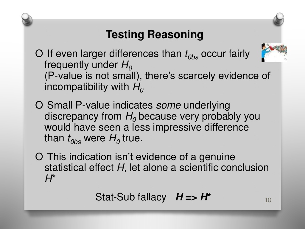
From inferring a genuine discrepancy from a test hypothesis, you can’t go directly to a genuine falsification of, or discrepancy from, the test hypothesis, but you can once you’ve shown a significant result rarely fails to be brought about (as Fisher required). The next stages may lead to a revised model or hypothesis being warranted with severity; later still, a falsification of a research claim may be well-corroborated. Once the statistical (relativistic) light-bending effect was vouchsafed (by means of statistically rejecting Newtonian null hypotheses), it falsified the Newtonian prediction (of a 0 or half the Einstein deflection effect) and, together with other statistical inferences, led to passing the Einstein effect severely. The large randomized, controlled trials of Hormone Replacement Therapy in 2002 revealed statistically significant increased risks of heart disease. They falsified, first, the nulls of the RCTs, and second, the widely accepted claim (from observational studies) that HRT helps prevent heart disease. I’m skimming details, but the gist is clear. How else is Gelman’s own statistical falsification program supposed to work? Posterior predictive p-values follow essentially the same error statistical testing reasoning.
Share your thoughts.
[1] Another relevant, short, and clear paper is Gelman’s (2011) “Induction and Deduction in Bayesian Data Analysis” (2011).
[2] You can search this blog for quite a lot on Gelman and our exchanges.
REFERENCES
Fisher, R. A. 1947. The Design of Experiments (4th ed.). Edinburgh: Oliver and Boyd.
Gelman, A. 2011. ‘Induction and Deduction in Bayesian Data Analysis’, in Error and Inference: Recent Exchanges on Experimental Reasoning, Reliability, and the Objectivity and Rationality of Science, Mayo, D., Spanos, A. and Staley, K. (eds.), pp. 67-78. Cambridge: Cambridge University Press.
Gelman, A. and Shalizi, C. 2013. ‘Philosophy and the Practice of Bayesian Statistics’ and ‘Rejoinder’, British Journal of Mathematical and Statistical Psychology 66(1): 8–38; 76-80.
Mayo, D. G. (2013) “Comments on A. Gelman and C. Shalizi:“Philosophy and the Practice of Bayesian Statistics”, commentary on A. Gelman and C. Shalizi “Philosophy and the Practice of Bayesian Statistics” (with discussion), British Journal of Mathematical and Statistical Psychology 66(1): 5-64.


")


A couple of comments. I think Gelman’s approach is a valuable twist on Bayes, in the spirit of Box. I had a go at applying it here: http://biorxiv.org/content/early/2016/10/25/072561
Having said that I think it’s worth taking Laurie Davies’ idea of ‘one mode of analysis’ seriously. Instead of: fit model using bayes, check fit using EDA, it is possible to instead incorporate EDA directly into the fitting criteria. One can and should of course vary the fit criteria during EDA.
The problem is that EDA is a somewhat awkward fit with both standard Freq and Bayes- I think a further conceptual shift is required. In particular I think probability theory plays a somewhat supplementary role, rather than a primary role. Again I’ve found Laurie’s work a good stimulus in this regard (though I’ve been trying to reformulate some of it).
Omcalaran:
Regarding the way that exploratory data analysis fits into Bayesian inference, see this paper from 2003:
A Bayesian formulation of exploratory data analysis and goodness-of-fit testing,
Click to access isr.pdf
and this paper from 2004:
Exploratory data analysis for complex models,
Click to access p755.pdf
I don’t think the fit is awkward at all!
Hi Andrew, thanks for the response. I’ve actually looked at those papers in a fair amount of detail and discussed them a bit with eg Laurie.
While I think both are nice papers I do think there is some awkwardness. Eg the mixture model example. Maximum likelihood blows up because it’s density based and regularising via priors doesn’t help much, as you note. A simpler approach seems to be to just measure fit at the level of the data/distribution function. Laurie has an example in his book, I’ve played around with a simple modification that seems to work well.
You could probably view it as a form of hierarchical model though, bringing it back into the Bayes fold.
Omaclaren:
You write, “the mixture model example. Maximum likelihood blows up because it’s density based and regularising via priors doesn’t help much…”
You read that wrong! Regularizing via _flat_ prior doesn’t help. Regularizing via informative prior helps a lot! See for example this paper from 1990: http://www.stat.columbia.edu/~gelman/research/published/electoral3.pdf
Hi Andrew,
Fair enough – my comment was probably too strong in that you can in fact very often find appropriate regularisers for almost all ill-posed problems, and express these in terms of priors.
What I was referring to, however, was this (Gelman, 2003, example 3.1):
>
“Unfortunately, this problem is not immediately solved through Bayesian inference….[you then give an example of a uniform prior, but don’t include any example using an alternative prior]…
…But now consider attacking this problem using the Bayesian approach that includes inference about yrep as well as theta…
…in either case, posterior predictive checking has worked in the sense of “limiting the liability” caused by fitting an inappropriate model. In contrast, a key problem with Bayesian inference – if model checking is not allowed – is that if an inappropriate model is fit to data, it is possible to end up with highly precise, but wrong, inferences.”
<
So what you suggest here is not to take (or at least not to prioritise) the 'regularisation via a prior' route (which I don't/shouldn't deny is possible) but to instead take a different route based on incorporating EDA.
What I am suggesting is that this is a general path available that, while it can of course work with both Bayesian and Frequentist inference, it potentially fits 'more naturally' into a different framework. This is of course somewhat a matter of taste.
Laurie's work can be seen as one such attempt to *start from* EDA. As I mentioned I played around with some small modifications of Laurie's approach and it seems to lead to a fairly simple approach that doesn't require careful choice of priors or the two-step 'fit, check' Bayesian approach to EDA.
So, I'm just trying to point out an alternative route to a similar set of ideas.
Thanks.
Not sure if you mean that sarcastically, but in either case ‘you’re welcome’ applies 😉
Omaclaran:
Intonation is notoriously difficult to convey in typed speech. In any case, I was not being sarcastic.
(see also Laurie’s comment further below, which I just noticed)
Om: Very interesting, I’ll study this further. Thank you.
Mayo, I would be surprised if Gelman felt that he was making “arguments against all Bayesian probabilisms” and so I find the first sentence of your comments difficult. Do you mean that he argued against every Bayesian probabilism? I don’t see that in his abstract. Perhaps you meant to say that he argued against probabilisms that are entirely Bayesian. (I’m not confident that I could define “probabilism”, but I think I get its gist.)
I also struggled with this bit in your slide: “This indication [a small p-value] isn’t evidence of a genuine statistical effect H, let alone a scientific conclusion…” I agree entirely with the final part, but I am not at all sure what “a genuine statistical effect” would be, and I can’t see how the idea that a small p-value is not an indicator of the existence of evidence regarding H. What is the relationship between the “genuine statistical effect” in the slide and the “genuine discrepancy” in the first sentence below the slide?
Michael: On the first, I defined probabilisms (in my PSA talk, so my comments use the term) as either probabilistic updating or Bayes factors or, for a non-Bayesian type, likelihoodism.
On the second, don’t forget the crucial requirement of Fisher’s that we not move from a single isolated p-value to inferring a genuine phenomenon. I’ve quoted it zillions of times–do you want a link? Sorry to be rushed, I have company.
I wouldn’t include likelihoodism as a form of probabilism since likelihood doesn’t obey probability theory, right?
Om: My intent is to distinguish the main roles probability is thought to play in statistical inference: to assess the support, probability, plausibility of claims given data–either with an absolute or comparative measure. That includes Bayesian updating, Bayes factors and likelihoodism. The other umbrella(s) involve using error probabilities (thus violating the LP). Most familiar is the use of probability to assess and control long-run error probabilities; less familiar is to assess and control the capabilities of methods to probe erroneous interpretations of data. The former is behavioristic, the latter is a severity assessment (sensitive to the data). The three P’s are: probabilism, performance, and probativism. Of course the labels don’t matter, but I find distinguishing probabilism vs the 2 error statistical methodologies of key importance.
For example,I happen to notice in the paper to which you linked, you refer to a “gold standard” theory of statistical evidence by Evans–a simple B-boost idea. I don’t know whose gold standard you have in mind, but it fails to satisfy the minimal requirement for good evidence. The central problem of scientific-statistical inference is the ease of finding a hypothesis to “explain” or fit the data. If H entails e, and e is observed, then you say e is evidence for H (unless H already had probability 1). Even though you wouldn’t even require entailment, it makes the point readily. That IS the central problem of reliable inference. If the probability of getting your B-boost for H is high,even if H is specifiably false, then H has passed with poor severity. In order to say that there’s good evidence for H, or that H has been well or even decently tested, you must show that you’ve probed flaws and found them absent. As Popper would say, you must be able to present your inference as a failed attempt to falsify H. That requires error probabilities, not mere B-boosts. That’s why confirmation theories (which are probabilisms) have all failed.
Yes I’m familiar with all that. I just think likelihood theory should be distinguished from probability theory since it doesn’t obey probability theory rules.
Anyway. RE Mike Evans and gold standards. I used scare quotes/actual quotes for ‘gold standard’, referring to his own statement in his book ‘the developments in this text represent an attempt to establish a gold standard for how statistical analysis should proceed’.
So, his gold standard at least (he is also a well-known statistician, in contrast to Popper, so must be allowed some claim to developing such standards!).
More importantly, I also distinguish evidence as it appears ‘within the model’ and model checking ‘external to’ the model, as with Gelman. So it is all consistent with Gelman’s falsificationist approach, it just differs from yours. It is only confirmationist ‘within a model’, as Gelman would say.
Anyway, take a look, check out the figures etc and let me know what you think.
Finally, as indicated above, I’m open to alternative approaches and am playing around with some attempts at improving the current best practice. It’s easy to criticise, but harder to be constructive. I can send you some attempts at improvement if you’d like.
I also referenced your work and controversies over statistical evidence there, for those who want to delve deeper. As it stands, it’s a paper using Bayes so it can’t really avoid being confirmationist ‘within the model’, despite having a falsificationist element ‘external to’ the model.
Om: Yes, I saw the ref, I think it was to the LP rather than anything on evidence, but I may have missed. It’s not a matter of being within or external to a model, I’m saying this is the case for anything that purports to be evidence. If little or nothing has been done to probe flaws with claim H, then a B-boost (or other even stronger fit measures) fail to provide evidence for H. (I’d qualify by degree of severity, but evidence is kind of a threshold concept–low severity is “bad evidence no test” (BENT). Not a little bit of evidence.
But the thing is, there’s no place along the hierarchical route you describe where this isn’t so, even though wide differences in types of problems and flaws are of concern.
Now your paper stops to talk about statistical evidence, and mentions that you’re surprised it hasn’t been settled. So that suggests you don’t consider it obvious. Moreover, I thought you were presenting it as an application of Gelman, and I take him not to be confirmationist. (I realize we’d need to go back and clarify terms).
I remain curious as to where the “gold standard” reference came from, I’m serious. Has it been called this, or were you simply meaning to express that you had it on good evidence (that Evans is solid on statistical evidence).
I don’t consider it settled in general, no. But that’s my own view.
I think Gelman would agree he is ‘confirmationist within a model’ and ‘falsificationist about the model’ in the sense that
– he uses Bayesian inference to pass from a prior parameter distribution to a posterior parameter distribution holding the model fixed
– this uses Bayes in the standard sense so is confirmatory by nature in the sense that the likelihood measures the change from prior to posterior support for the parameters
– Similarly Mike Evans defines the evidence, holding the model fixed, as the change from prior to posterior
But there is a falsificationist aspect in that
– both the prior and posterior parameter distributions imply predictive distributions in the ‘data space’ which can be checked
– if these don’t pass the checks then the posterior parameter distribution is suspect. That is, we can’t trust the ‘holding the model fixed’ part anymore so the ‘confirmations’ don’t mean much
– we use such misfits in the predictive distributions to ‘learn from error’ and improve our (now falsified/suspect) models
– this improvement is not governed by Bayes, or really any inferential procedure. More a creative ‘conjectural’ process a la Popper
I think this is all pretty clear in Gelman’s writing and in my attempt at applying it.
Having said that, I think there is potential for alternative approaches that take eg EDA more seriously and perhaps all forms of probability (even including error probs) less seriously
Om: It doesn’t make sense to say there’s no inferential procedure in Popper–the procedures for him are falsification and corroboration.
I was (quite clearly I thought) referring to the ‘conjectures’ part of ‘conjectures and refutations’ as in:
>
“In this way, theories are seen to be the free creations of our own minds, the result of an almost poetic intuition”
<
I believe this is consistent with Gelman's (consistent!) comments to you that he is not looking to 'infer new models' based on predictive checks. Rather he is looking to refute them and them think about new conjectures for better theories. These may be 'free creations of the mind'.
Om: poetic intuition is mumbo jumbo. Yes, we freely create, but for a refutation of H to be warranted, let alone to indicate a “better” theory, we need to vouchsafe an anomaly for H–a falsifying hypothesis. Read my comments on Gelman and Shalizi or search this blog for the series of posts on Popper.
Popper’s own words…I guess we pick and choose?
Anyway, RE:
“For a refutation of H to be warranted, let alone to indicate a “better” theory…”
This is where I would argue against your reading of Gelman. Or me. Maybe Popper, at least the good bits (since we can pick and choose!).
The point is that to me these are generally two separate tasks. Hence conjectures and refutations not confutations.
Also, I think an issue here is perhaps that many scientists who find some value in Popper often like the ‘conjectures and refutations’ part but not so much the ‘corroboration’ part. I know this is my view.
I think ‘corroboration’, like ‘confirmation’ can only really be defined ‘within’ a model, while ‘falsification’ can be defined somewhat ‘externally’ to the model.
Falsificationist Bayesians, and others, tend to restrict all measures of ‘confirmation’, ‘corroboration’ or whatever to ‘inside’ the model and take an almost purist ‘falsificationist’ approach wrt the model itself.
(Of course poetry is free to do as poetry does!)
This seems like a major source of miscommunication according to my reading of your reading of their reading of…Popper.
Om: The “free creation of the mind” was important to Popperians trying to fight the anti-realist logical positivists. No problem with being poetic, I just have no clue what work it was doing for your argument or position.
First let me say it’s fun to be conversing with you’all on my blog like old times. I’ve been rather stuck in my work, and will be for a while more. It’s nice to see people haven’t figured it all out yet, so there’s still a need for my book: Statistical Inference as Severe Testing.
I don’t identify likelihood theory and probability theory, OK?
OM: Anyway. RE Mike Evans and gold standards. I used scare quotes/actual quotes for ‘gold standard’, referring to his own statement in his book ‘the developments in this text represent an attempt to establish a gold standard for how statistical analysis should proceed’.
Cute. Does he mention how current day replication problems are based on supposing all you need is a B-Boost or the like?
In my book (which I’m so close to finishing) I set out what I regard as the most minimal requirement for evidence. Plenty of accounts won’t satisfy it—I admit that–and that’s what let’s us tell what’s true about them.
OM:So, his gold standard at least (he is also a well-known statistician, in contrast to Popper, so must be allowed some claim to developing such standards!).
Evans is a better source to learn about evidence than Popper? Hmm. Evans is all about belief change, Popper wanted no such thing. Still,Popper never gave us an adequate account of severity, falsification, or demarcation (all his babies)—improvements that my new book provides.
More importantly, I also distinguish evidence as it appears ‘within the model’ and model checking ‘external to’ the model, as with Gelman. So it is all consistent with Gelman’s falsificationist approach,
Again, you seem to be identifying “within” with confirmatory. This is perhaps in sync with Box’s use of Bayesian estimation within the model, but he uses “inductive” for model checking. Gelman does not.More terminological confusions.
OM:It is only confirmationist ‘within a model’, as Gelman would say.
Really? And does it take the form of a posterior probability or just estimating a parameter within a model? I took Gelman to be falsificationist/corroborationist. Maybe he’ll answer. But I have to repeat that these distinctions are entirely different from my talk of evidence which includes within, without, over, under, around and through.
OM:Anyway, take a look, check out the figures etc and let me know what you think.
A lot of it looks interesting, but I’d need to know more about the subject matter, and your goal in modeling it.
Indeed, likelihoods are not probabilities. Fisher is very clear on that point (and I could offer a link, but that might seem patronising 😉 However, perhaps they are among Mayo’s “probabilisms”?
Likelihoods do not comply with the standard axioms of probability so there is some danger in treating them as probabilities.
Michael: I already answered by reviewing probabilism, performance, and probativism. I sometimes refer to probabiisms as evidence-relation measures. Hacking uses “logicism” to describe much the same thing, and in 1972 declares he was all wrong to spoze there is any such thing as a logic of evidence or statistical inference. Blames it on being caught in the grips of logical positivism just 7 years before.
Mayo, I don’t need a link to Fisher, thank you.
Your response seems to miss my point entirely. I take Fisher’s advice as a way to avoid being overly influenced by misleading evidence, but I do not see how it is an answer to my question. Misleading evidence is evidence, potentially misleading evidence is evidence and weak evidence is evidence, so Fisher’s advice does not seem to justify your statement that “This indication [small p-value] isn’t evidence”. Are you using the word evidence in a dichotomous exists/does not exist sort of way? If so then you are not being very Fisherian.
Now you have written “genuine phenomenon”, “genuine statistical effect” and “genuine discrepancy”. I can see how the first and last might be interchangeable synonyms, but the meaning of the middle one escapes me.
Michael: LEW:Mayo, I don’t need a link to Fisher, thank you.
Well given what your wrote, I think maybe you do, so here it is:
i. R.A. Fisher was quite clear:
“In order to assert that a natural phenomenon is experimentally demonstrable we need, not an isolated record, but a reliable method of procedure. In relation to the test of significance we may say that a phenomenon is experimentally demonstrable when we know how to conduct an experiment which will rarely fail to give us a statistically significant result.“ (Fisher 1947, p. 14)
An isolated low p-value is not by itself evidence of a genuine effect or natural phenomenon. It comes from a post that also touches on the other issues we’ve been discussing. https://errorstatistics.com/2015/10/18/statistical-reforms-without-philosophy-are-blind-ii-update/
LEW: Your response seems to miss my point entirely. I take Fisher’s advice as a way to avoid being overly influenced by misleading evidence, but I do not see how it is an answer to my question.
What you say sounds nothing like Fisher and a lot like Royall. (So show me a link from Fisher.
LEW: Misleading evidence is evidence,
potentially misleading evidence is evidence and weak evidence is evidence,
Oh my god, when all your evidence that Mark is guilty is misleading you still have evidence??? When your evidence that Mark is guilty is misleading because you discovered the loot in his car, which you thought was his, but actually was deliberately dropped in his car by someone who wanted to frame him; and in fact your info that Mark was in the country that day was a lie, he wasn’t; and further, it turns out he doesn’t speak Spanish and you were misleadingly told he did; and you know the guilty person speaks Spanish–you don’t have evidence for his guilt (but actually evidence of his non-guilt).
Misleading evidence for H (in this case Mark’s guilt) is NOT evidence for his guilt.
LEW:so Fisher’s advice does not seem to justify your statement that “This indication [small p-value] isn’t evidence”.
I said it’s not evidence of a genuine phenomenon. You may take it as an (unaudited) indication of some discrepancy from a null, but not if it’s misleading (like when it came from the liar trying to frame him).
LEW:Are you using the word evidence in a dichotomous exists/does not exist sort of way? If so then you are not being very Fisherian.
That we qualify evidence and severity of tests, doesn’t mean lousy or misleading evidence of H is evidence of H. Not by my book, and not by Fisher’s. A probabilist may say it is.
LEW:Now you have written “genuine phenomenon”, “genuine statistical effect” and “genuine discrepancy”. I can see how the first and last might be interchangeable synonyms, but the meaning of the middle one escapes me.
I’ve explained Fisher’s sense of genuine phenomenon above. You must mean that the second and third are interchangeable. They are all intimately related, only Fisher uses “natural” in the above quote.
Mayo, I do not disagree with your position that inference should take into account the reliability of the evidence and the reliability of the report of evidence.
I know that you have several times refused to supply any definition of what you mean when you use the word “evidence”. That’s OK, I guess, but it is definitely not helping this conversation.
In general you do not know when evidence is misleading or non-misleading. Thus your example with the innocent Mark is not very appropriate. If it comes to light that Mark has been framed then the evidence is disregarded because it is misleading. You could also say that the true nature of the evidence has become clear and the assumption that the evidence pointed to Mark’s guilt was faulty. Either way, in the absence of knowledge of a frame-up and Mark’s alibi the evidence existed and had an unknown state of misleadingness. Is it better to say that it is extinguished by other relevant discoveries (frame-up and alibi) or that it changes or that it is discounted? I don’t know, but I do know that it is not helpful to suggest that it never existed in the first place.
Coming back to the original issue, it is a nonsense to say that a single small p-value is not evidence. The evidence may be unpersuasive when its misleadingness is unknown, but it nonetheless stands as evidence. Otherwise your first two bullet points on the slide lose their clear common sense logic and common language meaning.
Finally I note that even though you claim to have explained “genuine effect”, that is not the phrase that I found unintelligible. You have not attempted to explain what you meant by “a genuine statistical effect”, so you are being evasive.
Again, I do not disagree with your position that inference should take into account the reliability of the evidence and the reliability of the report of evidence.
Michael: i’ve defined evidence for a claim zillions of times: x provides evidence for H only if (and only to the extent that) H has severely passed a test with x. This is a falsificationist approach, but we can also corroborate (i.e., provide evidence for) H when we’ve subjected H to a stringent test, yet we fail to falsify it. We infer the absence of errors that have been ruled out with severity; we infer the presence of errors or flaws in H by falsifying H. For details check my published philosophy of science papers (below the statistics papers on my publication page).
Mayo, so observational data is not evidence?
re: the evidence issue.
I personally think it makes sense to have concepts of both
– evidence
and
– reliability of that evidence.
Royall’s approach seems reasonable in this sense.
Classically, you could say something like
– the normalised likelihood function is a measure of (relative) evidence
– confidence intervals are a measure of reliability of evidence
Having said that, confidence intervals are usually formed for particular estimates, e.g. you could form a confidence interval for the maximum likelihood estimate. You don’t usually form ‘confidence intervals’ for the whole likelihood function…
But then, asympototically (under regularity etc conditions), you can get confidence intervals by taking into account more of the observed likelihood function than just its maximum values – e.g. the observed Fisher information etc.
So its arguable that once you’re in the usual range of asymptotic validity, the whole of observed likelihood function itself – or approximating it using derivative information – already provides an approximate measure of the ‘reliability’ of evidence. A lot of the confidence theory is just ‘adding back’ information that it lost when it replaced the likelihood function as a whole with a point value.
Isn’t this the point Fisher once (or more than once) made?
In general, however, it is probably better to have a measure of reliability that includes in addition some ‘sample space’ derivative information a la Fraser et al and higher-order likelihood theory. So some at least vaguely frequentist reasoning, in the sense of ‘what if the data were different’, still seems relevant for defining an idea of reliability of evidence.
[Based on my current evidence I suspect Michael will roughly agree, while Mayo will object…but still, this current state of evidence may not paint a complete picture of the future so I could be wrong!]
Dr. Mayo, thank you for this post.
I’ve been interested in evidence since my college years through Evidence-Based Medicine (EBM). At first it was just a technical thing I had to do. I had the patient, I had to read the studies, appraise their validity and make a decision taking into account evidence, patient preferences and values. As I got older I dug deeper into the concept of evidence in the context of EBM. Some of the questions I have now originated from this blog and its comments section (thanks to all for that).
In EBM we make decisions based on the “best available evidence”. This is why it is curious that you mention the WHI case. There were reliable results (reliable as in consistent) from observational studies, that showed the benefits of hormone replacement therapy (HRT) on coronary heart disease (CHD). I would have to double check, but what I remember is that most of these studies showed a statistically significant result. Although we know observational studies are prone to bias, we regarded the hypothesis of HRT’s benefit on CHD as ‘very likely’ because of the consistency of results. We would need a very large amount of information to convince us otherwise. And a clinical trial (experiment) was not feasible for the longest time.
When it actually became possible (WHI) one of the major reasons to make it happen, and I quote, was “because the hypothesized cardioprotective effect of HRT cannot be proven with observational studies alone” (Controlled Clinical Trials 1998 19:pp 68). In my opinion, this was not about putting a hypothesis to a test, it was about the confirmation of the benefits of ERT on CHD beyond any reasonable doubt. Colloquially speaking, there was an urge to nail this hypothesis.
At the time, some found the study to be unnecessary, even unethical, just another stunt of the pharmaceutical industry. The worst case scenario was that HRT didn’t have any effect. That’s why the results were so surprising. Definitely, an experimental design with that amount of data was a severe test on that hypothesis.
The thing is that it had to come down to a mega-trial with massive amount of data to prove us wrong.
Yesterday, one of my colleagues posted the results of a Cochrane systematic review that concludes that there’s poor evidence in favor of a certain diagnostic test. That there would have to be, again, a large amount of data to prove that it actually works.
https://cochranechild.wordpress.com/2016/11/28/emergency-ultrasound-based-algorithms-for-diagnosing-blunt-abdominal-trauma/
In Medicine we are limited by sample size and stringent rules in clinical studies. Sometimes conducting an experiment is not possible on ethical grounds and we have to rely on observational methods. Sometimes it is too expensive. So we have to believe in the “best available evidence” and make decisions on that basis. Now this “best available evidence” could be potentially misleading but it is not likely that these hypotheses are going to be severely probed.
So, I guess Mr. Lew could be onto something when he says potentially misleading evidence is evidence.
Regards.
Martin:
He’d said that misleading evidence for a claim H was still evidence for H. The issue of having to make a policy decision with inadequate evidence is distinct from what I’m talking about in characterizing good/bad evidence and warranted/unwarranted inference. It’s true that when a theory has stood up to much testing, as for example Newton’s theory of gravity, yet later on that theory is falsified, we might say that the pre-Einstein evidence warranted many well-known experimental effects within Newtonian regimes (which is good enough for most purposes), but that it failed as evidence of the underlying gravitational process, which is about space time and not attractive forces. You can’t have the same data count as evidence for GTR and for not-GTR. In my work, I distinguish between “levels” of a theory, so that one can say that errors at a given level were ruled out with severity with x, but x failed to severely probe the phenomenon at a deeper level. There’s no problem for me in saying that data that had been taken in support of now falsified theory H can still be said to have gotten some things right about the phenomenon in question.
As for HRT, you are right that:
“At the time, some found the study to be unnecessary, even unethical, just another stunt of the pharmaceutical industry. The worst case scenario was that HRT didn’t have any effect.”Yes, they were all anxious to keep selling us on the need to take HRT to remain “Feminine Forever”.
Science progresses and claims thought to be based on decent evidence turn out not to have been. With HRT, the biases (“healthy woman’s syndrome”) from observational studies should have been suspected. Granted in the case of statistical effects it’s more complex because some women might benefit, or so they’re arguing.
I’ll be reading on your account of evidence. Finally bought your book.
Mayo, the summary of my comments that you gave to Martin, “He’d said that misleading evidence for a claim H was still evidence for H”, might have few enough characters to be tweeted, but it omits all of the meaning of my comments. I know that truth is now not politically important in your country, but the discussions here should be better than that.
A more correct summary of my comments would be that evidence is reinterpreted or discounted or assumed to be extinguished by a later revelation of misleadingness, but where the evidence has an unknown state of misleadingness (as is most often the case) it is evidence. Even the results of a severe test can occasionally be misleading, and thus Fisher’s advice applies to such a result.
The origin of this set of comments was your final bullet point on the slide which implies that an isolated P-value is not evidence because it might be misleading. That is not correct, and in my opinion it does not follow from Fisher’s advice.
Gelman’s model (1) of Section 3.1 Finite Mixture Models of his Bayesian
EDA paper is a mixture of two Gaussian distributions
0.5N(mu_1,sigma_1^2)+0.5N(mu_2,sigma_2^). He emphasizes the presence of
singularities in the likelihood function and regards this as the main
problem and one which cannot immediately be solved through Bayesian
inference. One possibility he mentions is to calculate the p-values of
the Kolmogorov-Smirnoff distance between the data and samples simulated
under the predictive distribution.
This seems to me to be unnecessarily complicated. One requires a prior
over the four parameters. Simulations are required to obtain the
posterior and for each simulated posterior value of the parameters
further samples must be simulated to calculate the p-values of the
Kolmogorov-Smirnoff distance. Even after doing all this it is not
clear what the conclusion is.
The problems arise because of Gelman’s insistence of using a density
based formal analysis, likelihood + prior + posterior, coupled with a
distribution based EDA check, Kolmogorov-Smirnoff distance. He
switches between a strong density based topology and a weak
distribution function based topology. I agree with Omcalaran, the fit
is awkward, indeed very awkward.
The problem is well-posed and requires no regularization. The
singularities of the likelihood are completely irrelevant. One simple
way of analysing the data is to minimize the Kolmogorov distance, or better
still, a Kuiper distance between the data and the distribution function
of the mixture. The analysis is performed completely in a the weak
Kolomogorov topology, there is no switching from strong to weak. The
analysis will give those parameter values consistent with the data, an
approximation region, which may of course be empty. It can be extended
to a mixture of four with in all 11 parameters.
As an example I take a sample of size 272 of the lengths of outbursts
of the Old Faithful geyser. If the 0.95-quantile of Kuiper distance of
order one is used as a measure of adequacy, a mixture of two normal is
sufficient with p_1=0.663, (mu_1,sigma_1)=(4.365,0.440),
(mu_2,sigma_2)=(2.000,0.299). The Kuiper distance is 0.105, the
0.95-quantile is 0.106 so that the mixture is just adequate. The time
required was 0.57 seconds. If the 0.9-quantile =0.098 is taken as a
measure of adequacy a mixture of three normals is required. The Kuiper
distance is now 0.054 with a computing time of 25 seconds.
Here is a simpler example. Generate i.i.d N(mu,1) data x_n where the prior
for mu is N(0,1). The posterior for mu is N(n*mean(x_n)/(n+1),1/(n+1))
if my calculations are correct. As far as I understand Gelman one now
samples under the posterior to give mn and then generates
i.i.d. N(m_n,1) random variables and compares these with x_n. Put
n=1000, simulate drawing from the prior 100 times and for each
such simulation draw 1000 times from the posterior. The EDA part is
to compare the data x_n with data generated with mean mn. To stick
with the Kuiper metric this can be done by calculating the Kuiper
distance between the empirical distribution of x_n and the
distribution function of N(m_n,1). For each of the 1000 simulations we
calculate the empirical 0.1-quantile of the Kuiper p-value. This is
done for each of the 100 simulations of mu under the prior. The
resulting p-values are almost but not quite uniformly distributed over
(0,1) with a minimum, mean and maximum values of 0.003, 0.372 and
0.965 respectively. If instead of comparing the x_n with N(mn,1) one
compares hen with N(mu,1) then the same simulation gives values 0.084,
0.105 and 0.128. In other words the p-values obtained from the
posterior are inflated which is reasonably obvious as mn is closer to
the mean of xn as is mu. Why not simply compare the x_n directly with
the mu? To compare x_n with mn is weird.
Laurie: So what’s the upshot of doing it your way rather than his?
“If instead of comparing the x_n with N(mn,1) one
compares hen with N(mu,1) then the same simulation gives values 0.084,
0.105 and 0.128. In other words the p-values obtained from the
posterior are inflated which is reasonably obvious as mn is closer to
the mean of xn as is mu. Why not simply compare the x_n directly with
the mu? To compare x_n with mn is weird.”
Sorry not to get your drift,the point about the different topologies is interesting.
Laurie:
Methods like what you can describe can work for simple problems. But for more complicated problems I prefer to write a full probability model. I don’t think it is onerous to supply prior distributions for real problems–typically this is a much easier task than setting up the “likelihood” or data model. And simulations are no problem at all–we can fit these models in Stan.
You can forget about the Kolmogorov-Smirnov thing; that was just a throwaway idea of mine that maybe didn’t make so much sense.
I come at this somewhat inbetween Laurie and Gelman so my attempt to bridge the gap:
There is no reason regularisation needs to be done in parameter space – it can also be done in ‘data space.
In fact I would argue this is what the point is of including yrep. Since the ‘likelihood’ is not ‘god given’ as all here acknowledge you could think of this as modifying the likelihood, or as a hierarchical Bayes model or something similar.
RE complicated: one thing that taking an approach more akin to Laurie’s approach is the possibility of including eg ‘checklists’, and other processes without simple expressions, into the model.
Although this way of using the terminology may not be popular around here, I personally like to use the word “frequentism” for an interpretation of probabilities that applies to data generating mechanisms (tendencies of occurrence of events under idealized infinite repetition – this encompasses also some “long run” propensity interpretations of probability) rather than for specific statistical methodology such as statistical hypothesis tests (although these are *based* on a frequentist interpretation of probability). In my interpretation, it’s a major characteristic of Gelman’s falsificationist Bayesian ideas that probabilities in them are interpreted in a frequentist manner (in my terminology). Yes, Bayesian ways of processing probabilities are compatible with a frequentist interpretation of probability (actually every frequentist knows this when in comes to multilevel data generating processes in which all the Bayesian computations refer to empirically observable distributions)! They refer to data generating processes rather than to (subjective or “objective”) epistemic assessments. Epistemic Bayesian (prior) models cannot be refuted (or undermined) by data because data is not what they model. Gelman’s models can be in conflict with the data because they are supposed to model the data.
One thing that I like a lot about “falsificationist Bayes” is that the Gelman & Shalizi-paper explained something that was implicitly, without proper explanation, done by many Bayesians before; I have seen many Bayesian papers in which the authors talked about their model as if it was a model for the “real” data generating process of interest while still referring to de Finetti or Jeffreys etc. for stressing the “coherence” of the Bayesian approach. But these concepts don’t go together very well. If you’re prepared to let the data reject your model, you cannot be coherent in the classical Bayesian sense.
Christian: Please explain what it means for Gelman’s priors to be frequentist. Does it allude to empirical Bayes–the distribution of theta, say, reflects how often theta takes various values? Or is it something else? In Gelman and Shalizi they suggest it can be any number of things, including beliefs. Pinning down the meaning of those priors would help a lot.
And since you’ve dropped by, which I’m glad,maybe you can explain in plain Jane language what Davies is saying in his comment.
“Please explain what it means for Gelman’s priors to be frequentist.”
See Sec. 5.5 here: https://arxiv.org/abs/1508.05453
Note that the main thing that is interpreted in a frequentist manner is the sampling model. In de Finetti’s terminology, the “prior” is the whole model as chosen before data, which includes the sampling model. What you probably mean by “prior” is what I call “parameter prior”. The arxiv paper lists three ways to interpret this, only the first of which is frequentist. But even if only the sampling model has a frequentist interpretation, one could still test it with misspecification tests that are independent of the parameters and therefore don’t depend on the parameter prior.
The main point of what Davies is saying regarding Gelman’s approach is that there’s some trouble with Gelman’s mixture example as analysed by Gelman, and it can be analysed in a better way not using a Bayesian approach and likelihoods. The major issue seems to be the potential degeneration of likelihoods in the mixture model, which Gelman addresses using “Bayesian regularisation”, i.e., clever choice of priors, and Davies states that no regularisation is needed if one doesn’t insist on analysing this using likelihoods.
Christian: I knew you’d explain the points at issue in a way that I can understand, at least approximately.Thanks.
Let me say that I noticed in your link some points on severity. The severity associated with a claim H is never the same as a test’s power at H.
The following is OK:
“The severity principle states that a test result can only be evidence
of the absence of a certain discrepancy from a (null) hypothesis, if the probability is high, given
that such a discrepancy indeed existed, that the test result would have been less in line with the
hypothesis than what was observed.”
However, it feels like a struggle, and is only one type of case. I’ll keep to it.
In a statistical test, agreement between data x and Ho is measured by test statistic T(x) such that the larger it is, the further the data are from what’s expected under Ho (in the direction of not-Ho)
Let the null Ho be mu ≤ 0 vs its denial H’.
Our interpretation goes beyond these preset hyps; it will be in terms of magnitudes of discrepancies from 0.
You observe t(x).
In your example, t(x) is considered evidence of the absence of a parametric discrepancy d from Ho.
That is, x is taken as evidence that mu ≤ d.
x provides maximal evidence for mu ≤ d if a larger difference than t(x) is guaranteed if mu > d. This is a deductive falsification of mu > d.
Replace “maximal” with “good” and “guaranteed” with “highly probable” and you’ll have the claim you want.
.
Christian:
“If you’re prepared to let the data reject your model, you cannot be coherent in the classical Bayesian sense.”
When I had a blogpost on “can you change your Bayesian prior” https://errorstatistics.com/2015/06/18/can-you-change-your-bayesian-prior-i/
nearly all the Bayesian responses were “of course”. Senn’s allegation that they were being incoherent was pooh-poohed as some fuddy-duddy de Finetti stuff. Dawid said there was nothing wrong with discovering you were wrong in expressing your beliefs, at least according to his slightly Popperian Bayesian approach. (This is how he deals with that “selection paradox” in a discussion by Senn).I hear of subjective elicitations that are corrected by the eliciter together with the elicited. Greenland talks about pointing out, using the data, that you can’t really have that prior.
They may all be comitting temporal incoherence, but that doesn’t seem to go hand in hand with regarding the prior as describing the parameter generation mechanism. And if they did want to see the prior as capturing the parameter generating mechanism, they’d be testing the prior with a single instance: the parameter(s) generating my data. As you often point out, that’s testing with a sample of 1.
Plus we don’t know we’ve selected our parameter randomly.
Of course if it’s really empirical Bayes, along the lines of Efron, say, that’s something else (although I don’t know that he does testing of priors). Anyway, I don’t hear Gelman viewing his approach that way, although it could be one possibility. Instead I hear him saying the parameters are fixed and our knowledge of them is random. I think he has in mind something like weight of evidence, at least when the prior isn’t merely a pragmatic ingredient. He can weigh in.
I see no difference between falsification and confirmation. Both are types of inductions but the former just uses a slight-of-hand and claims that if one fails to falsify some general theory then it’s status remains the same before as a “candidate for truth.” But that “candidate for truth” is a fallible one. In other words, falsificationists want to treat it as a truth to be able to generalize like a truth and avoid the problem of induction, but it isn’t really a truth because it is fallible! There is no difference here from induction! But it is a crude induction with no mention of any increase in the degree of support for the theory. Critical Rationalists idea of a well tested theory also requires this type of crudeness in induction despite claims it does not since one assumes it’s status has not changed when you need to use the theory for other things besides testing it again.
Bottom line is “so what if inductive inferences aren’t deductively valid”!
Here is another attempt at looking at “the problem of induction” (and Bayesianism) which seems more in tune with practice.
Click to access 1.%20Material%20Theory.pdf
Matk: I’ve written quite a lot on this issue, e.g., in ERROR AND INFERENCE (2010/11)-eespecially in my paper and my exchanges with Charmers and with Musgrave You can find those entries on my “publication” list in the left column of this blog. It’s definitely too complicated for a comment, however, if you search Popper on this blog, you’ll also get my position.
Thanks for the pointers and I am not a philosopher but a lot of what critical rationalist claim seems to me as dubious. Likewise, Hume’s problem of induction seems like small beer especially when no scientists consider that their theories as certain and assume fallibility in their work. I will check out your book as well. Also, I remember that you had a new book coming out. Will it cover these things as well? Thx.
Andrew Gelman: The mixture model is in no way ill-posed. You(!) make it ill-posed by your insistence on differentiating, a non-bounded linear operation with a tendency to produce ill-posed problems when
inverting, and having got yourself into this mess you have to be very careful with your prior to extract yourself. This is not a good example of Bayesian EDA, but it is a good counter example.
Mayo: I am not sure myself what to make of it. I am not sure what the goal is. As Christian Hennig pointed out, if the goal is to determine those parameter values if any which are consistent with the data you do not need a prior to do this. If your goal is to check your posterior then you do it the other way round: determine the parameter values consistent with the data and then evaluate the posterior at these points. Another possibility is that you don’t know where to look for consistent parameter values and calculate the posterior in the hope that it will move you in that direction. This is pure speculation. Even if that works sampling from the posterior will tend to concentrate around “very” consistent values and be sparse on the edge, the very opposite of what one wants. I had hoped that my simulations would be enlightening but they were not except for the latter point.
On the two topologies see Chapter 1.2.8 of my book. The “dogma” is to work in one weak topology as exemplified by the Kolmogorov metric or metric defined by Vapnik-Cervonenkis classes. You may already know this but just in case here is a link.
Click to access TR_145_%5B0%5D.pdf
Laurie:”As Christian Hennig pointed out, if the goal is to determine those parameter values if any which are consistent with the data you do not need a prior to do this.” So would you instead find max likely values for them?
Mayo:
Regarding, “if the goal is to determine those parameter values if any which are consistent with the data”: All this is conditional on a model for the data. And, as always, I don’t buy the argument that some model for the data is considered as God-given, but a prior distribution is not allowed. In my practice, the prior distribution is part of the model.
Andrew: To be fair, I don’t buy the allegation that error statisticians consider a model for the data as God-given. Isn’t that why people like Box say we need to use non-Bayesian significance tests for model checking? We have methods for model checking because we check models, not because we take them as God given (where does that come from?)
I don’t mind the idea of seeing a prior as part of the model–presumably, I guess, as a way to wind up where a likelihood would, if there were no nuisance parameters. I’d really like to understand how it works, as you know, which is really why I put together the PSA symposium, and ideally compare your way of modeling using priors to a non-Bayesian approach to modeling. I’m not trying to be critical. On the contrary, you’ve said you’re doing something akin to error statistics, so I’d like to illuminate the philosophical underpinnings. We always come back to to the meaning of the prior. In a comment (to this post) Christian says they are frequentist, which I don’t think I’ve heard you say before, except for the fact that you do say, from time to time, that the prior for a parameter in a model might be construed as the relative frequency of values found in an actual or hypothetical universe of all the times you or others have used the model, regardless of field. You said something like this at the railroad station in New Jersey
> I don’t mind the idea of seeing a prior as part of the model
David Cox and Nancy Reid definitely do as that implies prior and data are to be combined
“merg[ing] seamlessly what may be highly personal assessments with evidence from data possibly collected with great care,” and that maybe what a lot of the disagreement is about.
> relative frequency of values found in an actual or hypothetical universe
I preferred this one of theirs
“interpret the parameter prior in a frequentist way, as formalizing a more or less idealized data generating process generating parameter values” (Hennig and Gelman, 2016).”
My sense of Laurie is that they do not want to go past the data (or very far past) and that to me is too limiting. Also, I am already in a finite topology – anything we can observe is discrete and whatever generated that can be adequately represented finitely even if representations themselves (possibilities) are necessarily continuous. But I am looking forward to OM’s take on this.
Keith O’Rourke
Phan: I concur with Cox’s concern about combining disparate things, my point in the comment was simply to say, I’ll entertain Gelman’s proposed way of doing it and see where it ends up. There are, after all, frequentist matching priors, and Gelman says his approach can satisfy error statistical criteria. Calling it part of the model is merely semantics. Here’s what Cox and Mayo (2010) say: “Even if there are some cases where good frequentist solutions are more neatly generated through Bayesian machinery, it would show only their technical value for goals that differ fundamentally from their own. But producing identical numbers could only be taken as performing the tasks of frequentist inference by reinterpreting them” (p. 301) error statistically.
Click to access ch%207%20cox%20&%20mayo.pdf
Agree, if you only entertain priors that give those narrow “good frequentist solutions” then it is just semantics.
Its the restriction on “good frequentist solutions” such as uniform CI coverage for all possible parameter values that is causing the disagreement then. For instance, uniform CI coverage can lead to really poor type S and M errors.
Turning this around, one might consider how poorly priors that do lead to uniform CI coverage for all possible parameter values represent the reality you are trying get less wrong.
Keith O’Rourke
Phan: I still think it can be regarded as semantics, but it’s a confusing one. I would want good error statistical solutions, which differs from good long-run error rates.
Laurie: I’m intrigued that you’ve linked to something on Popper, but I’ve no clue as to how this is connected with the discussion in your comments.
The authors seem surprised that Popper denied you could have probabilistic guarantees about error rates*. They shouldn’t be. This was his key position, and it’s why he never succeeded in giving us an adequate account of severity. I take it as a point of pride that some well known Popperians (Chalmers, Musgrave)–who don’t do phil stat at all– say that my philosophy is like Popper’s except that I have a better notion of a severe test. Popper regards H as highly corroborated if it has been subjected to a stringent probe of error and yet it survived. The trouble is, he’s unable to allow that there are stringent error probes because they would requires endorsing claims about future error control. What these authors want (for a special learning theory context) is exactly what Popper says we cannot have.* That is why his ability to solve the problem of induction fails. I claim Popper’s problem is in not taking the error statistical turn. He once wrote to me that he regretted not having learned modern statistics (this is when I sent him my approach to severity). He was locked in the kind of search for a “logic” for science that logical empiricists craved (hence the disastrous theory of verisimilitude).
I’ve written a fair amount on Popper (e.g., in EGEK (1996), and in posts on this blog). But my new book “Statistical Inference as Severe Testing” (CUP)—nearing completion–has a lot of new reflections on Popper. They seemed necessary to make out the contrasts with my approach. I thought maybe that made parts of the book too philosophical, so I’m very glad if whatever message is behind your link is of interest to statisticians. Yet I’m clueless as to what it has to do with your recent comment. That is, what’s the connection between working w/ densities vs distributions (or however you put your point about Gelman) on the one hand, and Popperian falsification vs error statistical control on the other.Can you explain?
*They write: “there appears to be no way for Popper to speak about the reliability of well-tested theories, and yet one surely needs to be able to speak of one’s confidence in the future predictions of such theories”. Popper totally denies one needs to speak of any such thing. For him, an assessment of a theory’s degree of corroboration is merely a report of how well it has passed previous tests.
Andrew: As a challenge take the (some) Old Faithful data and give us the result.
Here is more complicated model: Y(x)=f(x)+epsilon(x) with the epsilon white noise, x in [0,1]. What is your prior over the sets of possible functions f? This has to take the number of peaks (we are interested in the number, size and locations of peaks) and the smoothness of f, say the existence an absolutely continuous second derivative. What is your prior? How do you calculate the posterior and what are your EDA checks?
Here a link:
Residual Based Localization and Quantification of Peaks in X-Ray
Diffractograms, Davies et al, AoAS 2008, 861-886.
http://projecteuclid.org/euclid.aoas/1223908044
See my book for further examples.
Take a simple model. The data x_n are i.i.d. N(mu,1) with mu N(0,1). Occasionally the mean of the data may be very large, a sort of outlier, and it is important to detect this. We use Bayesian EDA. The
dogma is first the prior, then the posterior and then the EDA. The EDA consists of comparing a mu generated under the posterior with the mean mean(x_n) of the data. Accept if |mean(x_n)-mu| <1.96/sqrt(n). For mean(mn) approx 10 and n=1000 the model would be accepted in about 90%
of the cases. So the order data-prior(model)-posterior-EDA doesn't work. The order ata-prior(model)-EDA does. If your Bayesian EDA doesn't work in a simple case why should I trust it in more complicated cases?
I have not applied my ideas to general hierarchical models and there is no guarantee that they will work. A joint paper with Omclaren is in discussion.
Mayo: Here is a simple example. You have data x_n and wish to know whether it is consistent with a normal N(0,1) i.i.d. model. Part of the check will be a question of shape. Does the empirical distribution function have the shape of a normal N(0,1) distribution function? To do this you calculate distance between the empirical distribution and the normal N(0,1) distribution using a metric. If you use a weak metric such as the Kolmogorov metric you will get a sensible answer. If you use a strong
density based metric, say total variation, the distance is always 1, d_{tv}(F_n,Phi)=1. So with a strong metric you learn nothing. In order to learn as in machine learning you need weak metrics. In order to
perform severe testing in this situation you must use a weak metric. Everything in my book is done in a weak topology. If you use Lebesgue densities then you must often regularize, as in minimum
Fisher information. In this situation a Bayesian prior will not regularize, the ill-posedness (sorry) is to deep for this to work.
Determining the parameter values is a numerical problem which can involve searches over grids. Sometimes easy bounds are attainable, sometimes one runs into a huge linear programming problem. Sometimes the problem you wish to solve is too complicated and must be replaced by a simpler one, for example replacing a global optimization by local optimization. In the Gaussian mixture example I start with a "mixture" of 1 and minimize a Kuiper distance. If satisfactory stop otherwise a mixture of order 2. The placing of the new component is decided using a high order Kuiper metric. Minimize again using a stepwise minimization routine. Continue until a satisfactory solution is reached. At the moment a mixture of 4 with 11 parameters is about my limit.
This is a minimum distance estimator. I never use maximum likelihood, I never use likelihood.
Laurie: Thanks, I’ll look for your book. I have a feeling Spanos would disagree with you. But I still am curious to know the connection to the link you gave about Popper and VC dimension. Was that just a vague metaphor for people doing or measuring
completelysomewhat related but largely different things?Dec 7: I altered the phrase because they’re not completely different. Popper’s simplicity/testability goal shares similarities with avoiding overfitting and achieving generalizability.
Laurie: I’m guessing now that your point is we can (and should) use non-parametrics to test assumptions. However, how do your answer Gelman’s comment: “Regarding, ‘if the goal is to determine those parameter values if any which are consistent with the data’: All this is conditional on a model for the data.”
Moreover, even the non-parametric tests of Normality depend on IID, don’t they?
Laurie:
As an example of this sort of thing see the time series decomposition on the cover of BDA3. We discuss issues of model construction, checking, and expansion for this example in the chapter on Gaussian process models.
phaneron0: Maybe I am misunderstanding you or possibly you me. Weak and strong topologies have nothing to do with the finiteness or otherwise of the space. Even if you only have discrete data you can have a weak topology or a strong one. Indeed the definition of a Vapnik-Cervonenkis class is based on a finite number of distinct points S_n={x_1,…,x_n}. Consider n points on the line and the set of intervals of the form I_x=(-infty,x] . Consider all subsets of S_n of the form I_x intersection S_n, x in R. There are exactly n+1 subsets, a linear function of n. If you consider finite intervals [a,b] you get n(n-1) subsets or something like that, anyway a quadratic function. If the number of subsets is bounded by a polynomial in n, say n^k. The family of sets is said to have polynomial discrimination. A metric based on such a family is weak. If you take replace the intervals by the family of Borel sets (taking things to the extreme) you get the all the subsets of S_n namely 2^n. This is not a polynomial in n. The metric based on this family of sets, the total variation metric is strong.
https://en.wikipedia.org/wiki/Sauer%E2%80%93Shelah_lemma
See also “Convergence of Stochastic Processes” by David Pollard for
applications in statistics.
Mayo: I am not sure what you mean by “just a vague metaphor for people doing or measuring completely different things”. I think Vapnik has a reference to Popper in his
The Nature Of Statistical Learning Theory
I skimmed through it over 20 years ago and seem to remember some comments on Popper. I take it seriously, indeed I think you must, and Vapnik takes it seriously. I am not a philosopher, I read it as a
statistician. I read Pollard’s book seriously.
Writing on phone on way to a meeting, but I think Keith means it in the sense of a ‘coarse discretisation of your sample space’.
Does this not work?
Laurie: I altered my phrase because they’re not completely different. Popper’s simplicity/testability goal shares similarities with avoiding overfitting and achieving generalizability. I was just slightly frustrated because you referenced something that I do understand in explaining something I don’t, and I got my hopes up that I’d see the link-up. But then there was no link-up.
I know Vapnik alludes to Popper in discussing V-C dimension, I heard him at a conference on simplicity. I understood his point, I simply don’t see the connection to your comment about Gelman, except as a vague metaphor.
Omaclaren: That is what I thought he meant and no it does not work. I can only repeat what I wrote before but try this. You have data always discrete, coarsen them if you wish as long as you still have the same number of data points although the occasional small atom doesn’t matter. Take the normal distribution function and discretize it to the same precision as your data. You now have two coarsened discrete distribution functions. The Kolmogorov metric will give you a reasonable comparison. The tv metric still gives the answer 1. Coarsening doesn’t help.
Mayo: Andrew uses likelihood, that is, densities in the mixture problem, he also uses the Kolmogorov-Smirnhoff metric which is a metric on the space of distribution functions. So he works with (i) densities (likelihood) and (ii) distribution functions (EDA). The two are linked, the distribution function defines a density, a density defines a distribution function as in
D(F)(x)=f(x), F(x)=\int_{-infty}^x f(u) du
with D the differential operator. Your metric in the F space must be weak as otherwise you cannot make meaningful comparisons. In the f space we can take the L_1 metric d_1(f,g)=int |f(u)-g(u)|du. The linear differential operator D from the F space to the f space is invertible but unbounded. In practice this means that d_1(f,g) can be very large but d_ko(F,G) small, in fact arbitrarily small. You
generate data at the level of the distribution functions F^-1(U) with U uniform on (0,1). Id d_ko(F,G) is small data generated under F and data generated under G will be close in spite of the fact that
d_1(f,g) is large. So my dogma is work in the F space using a weak topology which allows meaningful comparisons between different models and between models and data. This is necessary if you want to do severe testing, or Popperian rejection. If you work in the f space you can expect problems. These can be avoided to a large extent by regularization: my comb example and minimum Fisher information.
Yes, right. But what usually goes with this coarsening is the definition of likelihood as
density times discretisation scale.
ie a true probability not a density. Does this help at all?
(Yes I should probably be able to think this through by myself, but while we’re at it I may as well ask!)
Also, RE: ‘as long as you still have the same number of data points’ – do you mean as long as they are still distinct or as long as you still simply keep the same number of points even if previously distinct points become indistinguishable?
I think the point of the coarsening approach is to allow merging of distinct points, right?
And extreme case is to coarsen such that you only have one event left. Then all probability distributions would be equal.
So, very roughly, I think you argue for using distribution function based metrics because they generate the right sort of topology on datasets.
An alternative is to first define the right sort of topology on your datasets and then define (or convert) probability distributions over this a priori topology.
(This is what I was trying to do with my ‘likeness’ approach – c(x,x0) defines your metric/topology independently of your model).
omaclaren: “So, very roughly, I think you argue for using distribution function based metrics because they generate the right sort of topology on datasets”.
No, that is not correct. Given a family {\mathcal P} of probability measures on a space {\mathcal X} and a family {\mathcal C} of measurable subsets of {\mathcal X} one can define a (pseudo)metric on
{\mathcal P} by
d_{\mathcal C}(P,Q)d_{\mathcal C}(P,Q)=sup_{ C in {\mathcal C}}|P(C)-Q(C)|
I restrict myself to families {\mathcal C}{\mathcal C} of polynomial discrimination such as intervals in the case {\mathcal X}=R. Take {\mathcal C} to be all subsets of R which are the disjoint union of
intervals. Then d_{\mathcal C}(P,Q) can be expressed in terms of distribution functions as in
d_{\mathcal C}(P,Q)= \sup_{(a_j,b_j] j=1,2,..,(a_j,b_j] disjoin}\sum_{j=1}^{infty} F(b_j)-F(a_j)-(G(b_j)-G(a_j))|
This family is not of polynomial discrimination. None of the above requires any sort of topology on {\mathcal X}.
I can think of situations where data points may be merged perhaps to reduce the sample size but otherwise merging or truncating does not alter anything, or at least not anything substantial.
“An alternative is to first define the right sort of topology on your datasets and then define (or convert) probability distributions over this a priori topology. (This is what I was trying to do with my
‘likeness’ approach – c(x,x0) defines your metric/topology independently of your model). ”
In all but one of the situations I have considered c(x,x0) is defined over the respective empirical distributions, P_x and P_x0, the mean, the variance, the MAD, outliers, Kuiper distance etc. Sometime it makes sense to define a metric on the sample space but I have always derived the metric from P or P_x0, for example the Mahalanobis distance. I have never gone the other way round.
“No, that is not correct”
OK fair enough. I thought you said that at some point in your book.
RE merging, I meant count as another instance of the same value occurring, so not really reducing the sample size. Eg with a discretisation consisting of two ‘bins’ and the empirical measure each gets assigned the fraction of the original points lying in the bins.
But anyway, isn’t one of your main arguments that datasets that look similar should be analysed similarly, and since data is generated via distribution functions then this in fact is the main motivation for distribution functions – ie that similar distribution functions generate similar datasets. Rather than anything to do with distribution functions as such.
So I naturally wonder if you could go the other way – directly deal with ‘similar data’…which leads me to…
“In all but one of the situations I have considered c(x,x0) is defined over the respective empirical distributions, P_x and P_x0”
Yes this is something I slowly realised, and is in fact the main thing that makes me nervous. Is this really the right ‘level’ to compare models and data? There seems to me to be an ambiguity of the type ‘of what population is this a measurement’ here. But I still haven’t figured out where I stand on this, and how to articulate my vague intuition.
What do you do in small sample cases? Eg would you analyse a handful of data points (extreme case – one observation)? How would you justify your analysis or lack of?
Laurie and OM
What I was referring to was
“A more formal definitive of likelihood is that it is simply a mathematical function
L(; y) = c(y) Pr(y; ):
The formal definition as a mathematical function though, may blur that the likelihood is the
probability of re-observing what was actually observed. In particular, one should not condition
on something that was not actually observed such as a continuous outcome, but instead some
appropriate interval containing that outcome’ page 25 of http://andrewgelman.com/wp-content/uploads/2011/05/plot13.pdf
(Also see example at the very end from Radford Neal.)
Given that with such a definition, there is no likelihood derivative (in the standard sense), I am unable to grasp the issues.
I do accept that weak topology is the right topology for statistics and it would apply to discrete probabilities e.g. the intro example of a fair coin flip, where two observers differ in their sense of what is a head versus a tail, the coin flips always called differently by each are equal in distribution but not in probability.
Keith O’Rourke
The gaps in phanero’s function are thetas that failed to display.): L(theta ; y)=c(y) Pr(y ; theta).
So I think there is a definite ambiguity (interesting phrase, I guess) here.
Not sure if I can quite tease it out but I’ll try.
Given N iid samples x1,…,xN how do we interpret these?
Laurie I think interprets them ‘as a whole’ – one dataset to be approximated as one measurement of a ‘population’.
Hence differences between the given observation and any model generated comparison dataset z1,…,zn is really a comparison based on a difference measured by
C(y,y0)
Where
y=z1,…,zn
y0=x1,…,xn
Implicit in the iid assumption is that we disregard time ordering and hence the samples can be identified with their empirical distributions giving
C(P_z,P_x)
Implicit in the Likelihoodist approach on the other hand is that iid is a stand in for ‘measurements of the same object’. This came up in Keith’s comment above.
Now while the dataset might happen to be approximately decomposable into iid components, to be comparable to Laurie’s analysis – ie to be asking the ‘same question’ – we should again view the given dataset ‘as a whole’ ie as ‘one measurement’ y0.
Again we are lead to a comparison
C(y,y0)
So the point seems to be you can usually view a given dataset either as one instance of a whole – in which case ‘repetitions’ must be other objects of the same size (ie repeated instances of N dimensional datasets) or can be seen themselves as N repeated measurements.
Is there a general guide to when one view is preferable to another? I suspect that such ‘scale transitions’ ie viewing as a whole with properties measured by functionals of that whole vs viewing more as an aggregate of individuals depends very much on the question of interest.
Perhaps there is a connection to eg Simpson’s paradox, ecological fallacies – https://en.m.wikipedia.org/wiki/Ecological_fallacy etc?
And I suspect there is also some sort of bias variance tradeoff between the two perspectives – eg taking each xi instance as one definite measurement of a particular model can perhaps ‘take the model too seriously’ leading to overfitting and hence variability when the sample is varied, while treating it as a whole is a form of bias everything towards the population characteristics and not taking the individual aspects seriously enough.
omaclaren: I don’t think what you talk about is an “ambiguity”. I think that both views are needed. I assume that probability is interpreted in a frequentist manner (allowing some flexibility about what exactly this means, see my earlier posting). Then, in order to interpret what an assumption like “i.i.d.” means, you need to think of the whole dataset as a single instance of a data generating process (DGP) that generates whole datasets, because “i.i.d.” is a property of the full distribution of the whole dataset. On the other hand, the problem with this is that there is only a single instance of this DGP observed. So in order to learn anything from an effective sample size larger than one, there needs to be, within the model, some kind of “construction” of repetition. The i.i.d. assumption does this, it represents every single measurement as a replication of the others. It is possible to use non-i.i.d.-model such as time series models that still imply some kind of repetition, like assuming i.i.d. innovations or errors. It is also possible to define test statistics or Davies-style assessments of adequacy that test some expected “independence-features” of sequences assumed i.i.d., such as the runs test. Note that this is still based on implicitly assuming some kind of repetition, namely regularity regarding the runs length distribution. There are no omnibus tests of i.i.d., i.i.d. can only be tested against alternatives that have some kind of regularity that still allows to see repetitive “patterns” in the observed data. Testing i.i.d. against a general alternative would mean that the effective sample size can only ever be 1, because the whole observed dataset is essentially a single observation.
One off-shot of this is that in order to learn from data, probability models for data need to be constructed in such a way that there is some element of repetition in them in order to generate an effective sample size larger than one. This is regardless of whether replication is “real”.
Christian
> some element of repetition in them in order to generate an effective sample size larger than one
That is represented by a common parameter repeating in the likelihood.
>regardless of whether replication is “real”.
If replication was the reality (which you can hope but never know) you will gain with a common parameter, if its not, you lose big time (see link I gave for Simpson).
OM
Quickly Simpson’s would be dealt with along these lines http://andrewgelman.com/2016/09/08/its-not-about-normality-its-all-about-reality/#comment-303932
More generally and speculatively, my purpose is to get less wrong representations of reality with as much commonality (continuity) as possible while Davies’ purpose might be to keep all possible represeantions that are consistent with the data. In between might be Nelder’s search for a representation that maximise apparent commonness (e.g. his their are no outliers in the stack loss data set.)
Keith O’Rourke
omaclaren: “What do you do in small sample cases?”. There must be a story involved. How would I analyse n=1,x_1=2.567? Without a story, Iwould refuse. Take the copper example. With just vague information, the true quantity of copper is some where in the middle, I may offer two analyses, one based on the family of Gaussian distributions, the other, warned by the 1.7, based on M-functionals. Even if n is large, n=22000 for the S&P index the analysis will still be speculative to some extent as there are no comparable independent samples. The speculative element in statistics is always there.
“Given N iid samples x1,…,xN how do we interpret these? ff.” A full discussion of the points you raise would take much more space. Here is what I think I wrote. A model P is regarded as an adequate approximation to a data set x_n if typical samples X_n(P) of size n generated under P look like x_n. Similar statements have been made by David Donoho, Andreas Buja and Peter Huber, a sort of Swiss
mafia, and others. Thus comparison is not between each individual simulated data set and the real data sets but between a large number of data sets generated under the same P and the original data set. I do not make assumptions about the stochastic nature whatever of the real data set. The assumptions are placed on the model. If the model is i.i.d. then one can replace the a data set by its empirical distribution. However the ideas can be carried over to non-i.i.d. models, for example long range financial data mentioned above.
http://www.sciencedirect.com/science/article/pii/S0167947310002720
You can model the binary expansion of pi by i.i.d. B(1,0.5) knowing
that the the data certainly are not i.i.d. b(1,0.5).
Sometimes I think of populations when I have real data, the median income of a well-defined group of real people, but sometimes I don’t. I have no concept of population for measuring the copper content of a sample of drinking water: you have different samples of water, you have different degrees of contamination through other chemicals, you have different measuring instruments, you have different people taking these measurements, you have different laboratories with differing degrees of competence, collusion between laboratories, altering your data to reduce the variability, removing outliers before reporting the data etc.
Simpson’s paradox is an ever present danger.
Keith: I have not had time to read your paper in detail. On the example reported by (due to?) Radford Neal you cite him as writing “the inconsistency would go away if e was big enough”. That is the
inconsistency would go away if the continuous likelihood is replaced by F(h_i+e)-F(h_i-e) on a grid of
points h_i . This involves only the distribution function but leaves open the choice of e: if e is too small the inconsistency doesn’t go away. Why not use a minimum distance estimator based on the Kolmogorov metric? It is conceptually more elegant and requires no choice of e?
Laurie.
As long as the choice of e provides a finite discretization of the parameter space the inconsistency will go away.
Some choice of e better reflects the actual measurement processes that were undertaken (e.g. accurate to k decimal places and recorded to r decimal places).
The choice of e can be elegant – https://arxiv.org/abs/1506.06101
Keith O’Rourke
Mayo: “Popper regards H as highly corroborated if it has been subjected to a stringent probe of error and yet it survived. The trouble is, he’s unable to allow that there are stringent error probes because they would requires endorsing claims about future error control. What these authors want (for a special learning theory context) is exactly what Popper says we cannot have.* That is why his ability to solve the problem of induction fails. I claim Popper’s problem is in not taking the error statistical turn.”
I do not see how error statistics helps Popper and his followers with their problem. No matter how well designed I make my experiments, no matter what awards I get from others on these experiments, it all counts for nothing in the future. Why bother with designing them well in the first place? If I run very good test of a theory at time t1 that falsifies it and later on someone runs a bad test of the theory at time t2 which does not falsify it then which results should I choose? It seems like it would be the second test simply because it is the most recent. This seems absurd!
Mark: I don’t know where you learn your philosophy. Anyone who thinks we gain no reliable knowledge has a bankrupt philosophy of science. Error stat improves on Popper by showing how to achieve what he had in mind: we do indeed have self-correcting and error correcting severe tests. Popper regarded Peirce as one of the greatest philosophical thinker ever to have lived–his mistake was not learning quite enough from him. You can find my published work in the left hand column of this blog.
If corroboration is only some assessment of current or past performance but not of future performance then I have not reason why not to choose the most current test no matter how bad it is. This is not my stance nor your but it seems to me to be where critical rationalism ended up … and then died.
Mark: Popper did think he was stuck with a limited corroboration, but he was wrong. My philo of sci ≠ Popper’s. But he did argue it was most rationale to rely on the best tested theory, one that will teach us most, and point to break downs.
Sure he said that but his view being strictly anti-inductivist the way he claims then makes picking the latest test as i mentioned as much sense as any other test result. After all, a previous best test may have changed of status if you do not assume stability and project that status into the future. I think you even mentioned that in a previous comment. If you see that he really was an inductivist and do not buy into his rhetoric then his view is just a crude and distorted way of being and inductivist.
So do not get me wrong. I am 100% for designing the best tests possible and i am pro-induction.
The one wonder what use is falsification?
Mark: Replying properly would require at leas a short paper, so I won’y start: the rule here is, we don’t try to cram into a comment what’s been discussed at length in a post or a paper. Please see blogposts on Popper, and on induction and/or my PoS publications on my publication page (below the phil stat).
I keep scratching my head about Popper. He obviously did not contribute much if anything at all by his falsification notion since people knew things needed to be testable which by definition means they could be wrong. Long before Popper, scientists were well aware of confirmation/disconfirmation biases and controlling for measurement errors. So I still see him as under the spell of his own theory and in deep denial that it like most if not all approaches to supported beliefs require induction. Slight of hand is really what characterizes Popper and his critical rationalist followers.
Mark: Popper himself said the idea that falsification is the engine of science was obvious; even the amoeba performs conjectures and refutations. Enumerative induction from “given” observations–which all the logical empiricists accepted — was wrong. Few agreed with Popper and continued with logics of confirmation. Maybe instead of scratching your head you should read him? Begin with the first 50 pages of Conjectures and Refutations. I’ve written several posts on Popper bringing out the depth as well as the shortcomings. He’s one of a small handful of philosophers of science worth reading.
That was picked up on Popper’s Wiki page
He retired from academic life in 1969 ….
In Of Clocks and Clouds (1966), Popper remarked that he wished he had known of Peirce’s work earlier.
Keith O’Rourke
Phan: I don’t know of a quote to that effect, do you? The only quote I’ve seen is Popper saying something close to: Peirce was one of the greatest philosophical thinkers, and to indicate how obscure that quote is, I only came across it a few years ago.
phaneron0: I have only had time to quickly glance at the Miller-Dunston paper. Here some remarks in the light of their paper.
I do not place assumptions on data, a remark I have made before. I ask whether the data can be adequately approximated by the model under consideration.
Their Figure 1 gives a sample from a mixture of two skewed normal distributions to which they fit a mixture of normal distributions. The number of components they obtain stabilizes at two, that is the claim and is correct for n=10000. A glance at the data and the mixture for n=10000
shows that the two are not consistent. This is intended. The authors are interested only in the number of peaks and in this particular case number of peaks = number of components. If one wants to accurately approximate the skewed normal mixture more and more components will be required “obscuring the two large groups corresponding to the true components”. All very strange: miss the target but not by too much and here is a method for doing this.
The problem is, as I have mentioned before, the ideological requirement to differentiate. The operation is linear, invertible but unbounded and can cause problems as with Gelman’s mixture example. Gelman “regularizes” using a prior, Miller-Dunston regularize by discretizing. These are simply ad hoc strategies to solve a problem of their own creation. They allow for the “true” data generating mechanism P_0 not being a member of the parametric family but does anybody seriously think that the true data generating mechanism can be exactly described by a single probability measure? Their relative entropy c-posteriors even requires P_0 to have a density! The theory
consists of asymptotics with, as far as I can see, no attempt to check uniformity of convergence or with an error term for finite n. Of course this does not only apply to the Bayesians, Huber and Tukey have some pertinent remarks on asymptotics. I confess also to having done non-uniform asymptotics but only at the insistence of referees.
To return to their first example. Why not a minimum distance estimator? This is ideologically simply unacceptable and hence the search for regularizing strategies. Here is how I do peaks in one dimension. Take an epsilon Kolmogorov neighbourhood of the empirical distribution and
consider the taut string through it. Theorem: the taut string minimizes the number of local extremes of all functions in the epsilon neighbourhood. Moreover it can be efficiently calculated with an O(n)
algorithm. For a sample size of one million=10^6 the time required is 0.4 seconds. The taut string is a linear spline, the density is piecewise constant, but if all you are interested in is the number, location and size of the peaks your job is done. If you want a smooth density you will require some more time, in total 184 seconds but this depends on how smooth you want the density to be. There is no
assumption about a “true” data generating mechanism, no P_0, no priors on the number of peaks which can be zero, for example data generated by an exponential distribution which makes it impossible to use a mixture of normals. It is fast and interpretable. The radius epsilon of the Kolmogorov neighbourhood is specified by the user, who may be satisfied with an error of 0.005 or even 0.01 or may use the 0.9 quantile of the Kolmogorov metric for n=10^6, namely 0.0012. All
this is about ten years old and is covered in Chapter 10 of my book.
The authors mention convergence with respect to the weak topology. You also stated that you regarded the weak topology as the correct one for statistics. This is different from what I call a weak topology. The Kolmogorov metric is a weak metric but does not topologize the weak topology in the sense of Miller-Dunston. In fact no affinely invariant metric topologizes the weak convergence.
Mayo: “Laurie: I’m guessing now that your point is we can (and should) use non-parametrics to test assumptions”. No this has nothing whatsoever to do with it. Gelman claimed that my ideas would not work for more complicated models. I took non-parametric regression as an example of a more complicated model.
There are too many interesting comments now to reply to…
For now, a quick thought.
Laurie said
“You can model the binary expansion of pi by i.i.d. B(1,0.5) knowing that the the data certainly are not i.i.d. b(1,0.5).”
At first I thought, sure why not?
But thinking again – I assume this means ‘at the level of empirical distributions’ eg the relative frequencies of digits. At this level then yes, that works fine. We have discarded the ordering and have no idea what follows what.
But as an ordered process then maybe not. Assuming we have a deterministic calculation process available to calculate the digits sequentially then the binomial data will not ‘look like’ the data to those who have access to this process and use this in their fit measure – we know what follows what. We may want to fit the actual ‘underlying dynamics’ not just the time average/ensemble average.
In the later, dynamic (or ‘micro’) case we have a probability distribution with a parameter for each location in the expansion.
In the former, ‘static’ or ‘macro’ case we have a single parameter for the ‘population of digits as a whole’.
I have probably not expressed this particularly well but I think the basic point connects back to what I still think is a legitimate ambiguity in the discussions and also to Keith’s comments about repeating parameters, Simpson’s paradox etc.
Perhaps one way to summarise is to say that there seems to be an issue of having different coarse grainings of interest and subsequent incompatibilities of these once chosen (see again Simpson’s paradox, Keith’s comments).
Also, as another side comment, while I agree that naive differentiability etc assumptions are bad, it is also very difficult to do science without some concept of how one quantity varies as you vary another. There are also numerous ways of generalising the mathematical concepts to make things work.
Perhaps it’s just a coincidence but RE my above comment I note that it’s difficult to think about ‘dynamics’ without a notion of ‘difference’ or ‘derivative’ or ‘variation’. So again, it depends on the level of detail that’s of interest.
It may be possible to think about a coarse grained distribution and discard the underlying structure, but many scientists also want to go beyond that and are willing to entertain stronger assumptions to guide them. It should of course be emphasised when exactly we are making stronger assumptions.
I wonder – would we know much about geometry if we just cared about things like the relative frequency of the digits of Pi?
Terence Tao speaks of the fundamental dichotomy and interplay of structure and randomness, and I agree – you need both.
omaclaren: In the case of the binary expansion of pi the modelling includes the conditional probabilities, p(0|1),p(1|1), …., p(0|11111), p(1|11111), p(01|1), and so on up to whatever order makes sense for your sample. You can also make bets, give odds for the number of zeros from n:(n+m) although you have not tested this set. When you model in this manner you take the binary expansion in the order given. As far as I am aware the binary expansion of pi has passed all tests for independent in spite of the fact that pi is not a complex. This is not to say of course that it will eventually fail such a test. Perhaps I didn’t make it sufficiently clear but I was not just talking about the relative frequency of zero and one.
Whatever, given such data you have no way of knowing whether it is deterministic chaos or random. How do you determine the dynamical law governing the binary expansion of pi if you only have the data and you do not even know that pi is involved? Bohmian mechanics is deterministic chaos as is the simple coin toss. You know the underlying dynamics of coin tossing, Newtonian mechanics, but the system is chaotic, a small change in the initial conditions alters the result. In spite of knowing the dynamics you cannot use them to forecast the result because you do not know the initial conditions. Thus in spite of this you model the throws as i.i.d. There is some work by Salem and Zygmund (?? I think) on lacunary trigonometric series for which obey central limit theorems, that is look random.
I prefer described data as chaotic rather than i.i.d.
My comment on Simpson is that you may have a Simpson type paradox without being aware of it. Your data set is not homogeneous but you don’t know this because your don’t have the relevant data. Take the Berkley example on male and female students with no information on the individual courses.
If you model dynamical systems, say Brownian motion, which involves a concept of velocity then you will probably build differentiability into it although Brownian motion is non-differentiable. I have no objections to this. The examples we were discussing, Gelman’s mixture and the article on Bayesian coarsening Keith do not fall into this category. There are no dynamics involved, the problem is easily solved by a minimum distance estimator and yet this is simply unacceptable from the Bayesian-likelihood point of view. In the case of peak detection the taut string is very fast, less than 1 second for a million observations, and there is a theorem but it is completely unacceptable from the Bayesian-likelihood point of view.
RE deterministic chaos vs random.
Yes I agree in that there is no real distinction between the two (perhaps with some exceptions).
Despite that I think scientists are very often interested in discovering possible dynamical ‘laws’. In particular some kind of synthesis between ‘mechanism’ and ‘statistical’ aspects.
Last time I checked (it’s been a while) models for things like population cycles of foxes and rabbits that incorporate simple yet ‘wrong’ mechanistic assumptions (eg Lotka Volterra) outperform those based on purely statistical modelling. A combination of the two aspects is often successful and desirable.
So again, I don’t think it’s as simple as, say, giving up on thinking about underlying mechanism because of complexity or conversely thinking there must be one true mechanism. One of my favourite popsci books (with some amateur philosophy) is https://en.m.wikipedia.org/wiki/The_Collapse_of_Chaos
which is written by a biologist and a mathematician. It has a number of interesting discussions of the interplay between the simple and the complex.
What I would like most from your approach is a better idea of how to incorporate such hypothetical mechanistic assumptions. It is clear in Gelman’s work how to do this.
Similarly almost all work on constructing and parameterising mathematical models that incorporate both mechanistic understanding and statistical understanding in biological systems seems to be either Likelihoodist or Bayesian.
So there does seem to be something to the conceptual view of these approaches that fits with the scientific modellers mindset. Perhaps this will change.
I recently sent you an example of ion channel gating modelling and estimation. I still want to know how you might tackle such questions (funnily enough for readers of this blog, David Colquhoun made his name in part based on using likelihood methods to fit such data to mechanistic models of channel gating).
I believe these sorts of examples are what Gelman means by ‘complicated’ – the need to incorporate layers of mechanism – rather than say nonparametric regression.
RE Simpson. Again this is similar. The danger is ever present and the only ‘solution’ is to be willing to consider potentially wrong finer scale analyses. Pearl explicitly argues Simpson’s paradox requires causal reasoning to resolve. Again what I struggle with in your approach is where and how to incorporate mechanistic or causal assumptions as opposed to just representing the observable data better. I don’t think this is something to give up on, but perhaps you disagree?
RE the minimum distance estimator. I have no objection to this but for the sake of argument I would say – many people, especially Likelihoodist and Bayesians simply don’t think in terms of ‘estimators’ and perhaps with some justification. I also view ‘minimum’ or ‘maximum’ criteria more as ways of defining or characterising something than ends in themselves. So the justification is not in general immediately obvious.
For example, when I put on my Likelihoodist hat I am thinking in terms of ‘which models (parameter values) are consistent with the event I observed and to what degree’. One can use different ways of defining the ‘event observed’ – eg condition on a neighbourhood of the empirical distribution – but the conceptual view is clear. The advantage I think is providing a clear framework. Of course the user must fill in the details of ‘event observed’, ‘models under consideration’ etc but this is where the thought comes in.
So I wouldn’t say Bayes or Likelihood or whatever are ‘right’ or ‘wrong’ I would say they are frameworks for statistical inference whose success or failure depends on how we fill in the details.
Similarly Newton’s second law is really a framework, the success of which depends on our ability to find appropriate and general enough force ‘laws’.
So the question to me is – what is your approach a framework for? Can it incorporate mechanistic or causal assumptions? Can it approach the same class of problems that people use eg likelihood and modifications of likelihood for? Is the conceptual shift you argue for a price scientists would be willing to pay?
Or is it something that is more suitable for some particular class of statistician or ‘data scientist’ but not those interested in ‘mechanism’?
I think this is essentially what people like Gelman think – they don’t see how to incorporate their ‘bread and butter’ mechanistic modelling ideas into your framework.
[caught in filter again sigh…seems to depend on whether commenting via phone, or which browser I use…weird.
Mayo: Feel free to delete any duplicates.]
Another quick comment re: ‘level of description’, ‘repeating parameters’ etc. I just came across this work by Wang and Blei ‘A General Method for Robust Bayesian Modeling’:
Click to access 1510.05078.pdf
Without going into the details (which I haven’t read!) I note that the basic idea of ‘localisation’ :
>At its core, a Bayesian model involves a parameter β, a likelihood p(xi| β), a prior over the parameter p(β | α), and a hyperparameter α. In a classical Bayesian model all data are assumed drawn from the parameter…[β]…
> To make it robust, we turn this classical model into a localized model…
> …In a localized model, each data point is assumed drawn from an individual realization of the parameter p(xi | βi) …This is a more heterogeneous and robust model because it can explain unlikely data points by deviations in their individualized parameters…
>…In the localized model of Equation 1.2, however, each data point is independent of the others. To effectively share information across data we must fit (or infer) the hyperparameter α.
This appears to be the same sort of basic point that Keith and I were trying to make – the interplay between the level of description and robustness.
This is what I meant by:
> Implicit in the Likelihoodist approach on the other hand is that iid is a stand in for ‘measurements of the same object’. This came up in Keith’s comment above.
and Keith (I assume) in:
> Christian: some element of repetition in them in order to generate an effective sample size larger than one
> Keith: That is represented by a common parameter repeating in the likelihood
So the ‘localisation’ approach above appears to be saying each measurement is a measurement of ‘something else’, hence has its own parameter and no repetition (in the extreme case).
We of course then need to connect the parameters back together in some way to have enough data to estimate the parameters. (One way of course being empirical or hierachical bayes, which are also related to James-Stein estimators).
The trade-off between using one common parameter subject to ‘repeated measurement’ and as many parameters as data points each then subject to only ‘one measurement’ indeed appears related to robustness issues.
More ‘paradoxes’ seem related – Stein’s, Neyman-Scott etc.
So: level of description, ‘mechanism’ (or ‘structure’/factorisation etc) are all crucial issues here.
The commonness representation for hierarchical model switches from p(xi | β) and p(β | α) to p(xi | βi), p(βi | α) and p(α | tau) [and folks argue whether p(βi | α) is a prior or likelihood].
In order to get new knowledge, I believe risky representations need to made and severely tested.
Keith O’Rourke
Soory, again: We were (are?) discussing Bayesian EDA and Gelman’s approach to
it. One has a model(prior), calculates the posterior, samples for the
posterior, generates data from the result of this sample and then
perform EDA to see if the generated sample looks like the real
data.
Yes, back to that.
One ‘has a model’, which is a bit ambiguous in many ways (as discussed all over the place above).
I’ll try to write out things as explicitly as possible…might get messy. I’m sure Andrew can correct me if I go wrong, though my interpretation may simply be different.
To start, say, one has a standard Bayesian model consisting of two components:
[ p(Y|θ), p(θ|α) ]
[For some reason, Bayesians often refer to p(Y|θ) as the ‘likelihood’ or the ‘sampling model’, but I don’t really like either term. Obviously p(θ|α) is the prior with hyperparameter alpha, but it is also helpful to call this the parameter prior (as Christian mentions above).
Also, though these components are often discussed in density terms I think it makes most sense to make sure you are always dealing with true probabilities, whether via integration, definition of event of interest etc.]
You can put these components together to define a prior *predictive* model (to distinguish from prior parameter model)
p(Y|α) = ∫p(Y|θ)p(θ|α)dθ
which averages the ‘sampling model’ over the parameter prior. You can think of this as your ‘predictions based on the sampling model and the prior parameter model’.
Then you observe data y0.
You want to ‘update’ your predictive model ‘conditional’ on this observed data, i.e. you want something like
p(Y|α,y0)
This is somewhat ambiguous because it seems to say
p(Y=y|α,Y=y0)
which would seem (to me) to be 1 if y=y0 and 0 otherwise.
So instead you follow Gelman (say) and extend the model to consist of
[ p(Yp,Y|θ), p(θ|α) ]
where Yp represents what you *predict*, Y represents data that you either average over or condition on in order to make predictions – this should become clear in what follows.
The above gives an assumed decomposition of the joint distribution
p(Yp,Y,θ|α) = p(Yp|Y,θ)p(Y|θ)p(θ|α)
Here you could think of both Y and θ as ‘prior parameters’ and p(Y,θ) = p(Y|θ)p(θ|α) defining an extended parameter model. We further (typically) assume the structural condition
p(Yp|Y,θ) = p(Yp|θ)
which captures the idea that the parameter θ ‘summarises’ all information available for prediction.
So we have
p(Yp,Y,θ|α) = p(Yp|θ)p(Y|θ)p(θ|α)
For prior predictions we don’t know Y beyond its ‘prior’ p(Y|θ), so being proper Bayesians (here!) we average over it (along with θ), giving
p(Yp|α) = ∫ ∫ p(Yp|θ)p(Y|θ)p(θ|α) dydθ
but under the above independence assumptions this gives
p(Yp|α) = ∫ p(Yp|θ) ∫ [p(Y|θ)p(θ|α) ]dy dθ
The inner term is just
∫ [p(Y|θ)p(θ|α) ]dy = ∫ p(Y,θ|α) dy = p(θ|α)
so we have
p(Yp|α) = ∫ p(Yp|θ) p(θ|α) dθ
which is a lot of work just to get to the ‘usual’ prior predictive distribution.
Now, though, we can more sensibly address the updating of predictions. Suppose we observe
Y = y0.
We then want
p(Yp|α,Y=y0)
which makes much more sense than previously. We can follow the above reasoning again, but replace integration over arbitrary Y
∫ [p(Y|θ)p(θ|α) ]dy = ∫ p(Y,θ|α) dy = p(θ|α)
by integration over Y=y0
∫_{Y=y0} [p(Y|θ)p(θ|α) ]dy = ∫_{Y=y0} p(Y,θ|α) dy = p(θ|α,Y=y0)
So now we have
p(Yp|α,Y=y0) = ∫ p(Yp|θ) p(θ|α,Y=y0)dθ
as our posterior predictive distribution for Yp, as expected.
Now, EDA, model checking etc. This is the controversial/difficult part so naturally I’ll take the safe route and say very little.
At minimum you can simulate from p(Yp|α,Y=y0) by drawing from the posterior parameter distribution, plugging into the ‘sampling’ model p(Yp|θ).
Presumably your new predictions should be ‘pulled towards’ y0, so you want to check this. You plot Yp and y0. If you are holding all else fixed, e.g. α, the structural assumptions hold etc then in some sense you expect the variation of Yp *relative to* y0 to ‘look like noise’.
That is, the assumption is something like
p(Yp|α,Y=y0) ~ Noisy variation about y0.
E.g. in a simple case you might find
p(Yp|α,Y=y0) = N(Yp-y0,f(α))
or something along those lines.
The basic idea is that it is a sort of ‘residual check’. I am a little unsure of the full status of the ‘formal’ justifications at this point, however. It makes some intuitive sense, at least.
There are at least two typos/mistakes in the ‘derivations’ above, probably fixable. You get what you pay for 🙂
Laurie: Even if the generated sample doesn’t look like the real data, its hard to pinpoint the source–even w/o priors. Conversely, observed data can look like data generated by model M, even if there’s violations that show up in focussed tests of assumptions.
But maybe this is irrelevant since you said the discussion had nothing at all to do with model testing, in your last comment to me.
omaclaren: “What I would like most from your approach is a better idea of how to incorporate such hypothetical mechanistic assumptions. It is clear in Gelman’s work how to do this.”
I will try again, formulated slightly differently. I have the the data, the mixture or some other model maybe with mechanistic assumptions and search the whole parameter space to find those
parameter values if any which are consistent with the data. For the mixture model I use the Kolmogorov metric to check consistency. Gelman does not search the whole of the parameter
space but only that part obtainable from generating parameter values from the posterior. The main point here is not the posterior but that the search is restricted. For the mixture model, Gelman’s own example, He also checks consistency using the Kolmogorov metric. Why is his approach better, more natural, capable of including mechanistic assumptions and mine is not? This time if possible without an
introduction to Bayesian statistics.
“Now, EDA, model checking etc. This is the controversial/difficult part so naturally I’ll take the safe route and say very little.”
So maybe not so clear after all.
Mayo: It may well not be easy to pinpoint the reason for the misfit. It may be because of the data, Huber has some nice examples of this, or a completely different model may be required.
“even if there’s violations that show up in focussed tests of assumptions”
Do you have an example?
Gelman stated that my ideas would not work for more complicated models. I took non-parametric regression as an example of a more complicated model. That was all. It turns out he meant other types of
models.
Laurie: ” The main point here is not the posterior but that the search is restricted.”
I think that is the main point – the posterior hopefully provides a sensible restriction to facilitate empirical learning or perhaps better put getting somewhere beyond the data.
(Being just hopeful it needs to be tested.)
Keith O’Rourke
Yes – he is still carrying out Bayesian inference and so his candidate answer is of course based on the posterior. He just wants to check if it did in fact work. Possibly based on other criteria than that used to fit the model. You can also carry out out of sample predictive checks.
This basic idea seems quite reasonable and I’m unsure what aspect is unclear and how else one would explain it. In terms of the calibration and best way to carry out the checks, there is some controversy and better formalisation would help here.
I also noted to Gelman above that it is possible to try a ‘one mode’ analysis.
RE – ‘search the space to find values consistent with data.’
This is the same orientation as the Likelihoodist. It is unfortunate that many work with densities instead of probabilities but a number of people in that school – Sprott, Lindsey etc – point out that it is best to stick with probabilities. Everything is bounded etc. We have discussed the ‘coarsening’ approach, which event to condition on etc above. There is no reason likelihood or Bayesian folk can’t incorporate these ideas. I think the likelihood approach is a more natural fit than Bayes for a number of reasons that I won’t go into.
There are legitimate conceptual issues to consider regarding ‘what level’ to model the data at and the relation to various paradoxes. The Likelihoodist offers an interpretation and guidance (see eg Keith’s links and comments) for the paradoxes. I find this helpful.
As Gelman pointed out above, you can do nonparametric Bayes, though it is perhaps not as developed as alternatives.
Laurie-
Perhaps you could take one of Gelman’s hierarchical/multilevel regression examples and show how your approach works as well/better.
Don’t have an example immediately at hand but his BDA book and/or his multilevel modelling book (http://www.stat.columbia.edu/~gelman/arm/) have plenty of examples.
Also the reason for writing out the explicit ‘derivation’ above is that a) it was not clear to me how you were interpreting Gelman’s approach and b) a significant aspect of Gelman’s posterior predictive checks involves introducing explicit notation for data replications. I thought it would be helpful to discuss what he is doing using his own notation explicitly introduced for that purpose.
You have previously expressed puzzlement that what he is doing seems to lie outside of the standard Bayesian setup. Part of the answer, I believe, lies in his notation.
Om: you say “he is still carrying out Bayesian inference and so his candidate answer is of course based on the posterior. He just wants to check if it did in fact work.”
So far as I’ve seen, Gelman denies the product of his account is inference in terms of a posterior probability on a model/hypothesis, or a comparison of posteriors. Unclear what it means for it to have “worked”.
Here’s from his abstract on my blogpost:
“We can perform a Bayesian test by first assuming the model is true, then obtaining the posterior distribution, and then determining the distribution of the test statistic under hypothetical replicated data under the fitted model. A posterior distribution is not the final end, but is part of the derived prediction for testing. In practice, we implement this sort of check via simulation.”
Perhaps I should say ‘didn’t obviously fail’.
He has a prior parameter model and a sampling model (weird term yes). These imply a predictive model.
Bayes updates the parameter model. This implies another predictive model.
This latter quantity can be checked. It may not fit – eg Bayes offers no guarantee under misspecification. If it doesn’t look obviously bad we are temporarily happy with the Bayes result. The result of course being both parameter and predictive distributions. If it doesn’t fit then we are not happy with the Bayes result.
Is this part clear?
I find the basic scheme of Gelman very intuitively obvious but with perhaps some subtleties.
It may happen that the ‘intuitive’ scheme fails for one reason or another but I here I am struggling to get to a point where critics of Gelman demonstrate they understand the general aims.
Perhaps others have different intuitions and are immediately picking up on the subtle difficulties?
Om: “If it doesn’t look obviously bad we are temporarily happy with the Bayes result. The result of course being both parameter and predictive distributions.” This happiness mightn’t be warranted if it probably wouldn’t look obviously bad, even if there were misspecifications. Gelman and shalizi appear to agree, but it isn’t clear this is satisfied. Likewise, if it does look obviously bad, there’s a question about correctly pinpointing what’s responsible, what needs modification. I don’t see how Davies points relate to these issues, really.
Yes this is where the question of which checks to carry out – based on predictive distributions – is relevant.
There are other subtleties too.
But first everyone needs to be talking about the same thing so we can decide whether it is a ‘good thing’ or not.
Are you (and Laurie) comfortable with the concept of a posterior predictive distribution? (Regardless of whether it is used for testing).
I for one do not understand what is going on.
Let us take the Gaussian mixture example. Gelman writes that the idea is to limit the liability caused by fitting an inappropriate model. Suppose sampling from the posterior gives a good fit. He writes that in this case everything is fine as we have a truncated model which fits the data well. We can all discuss what he means by a truncated model. Suppose that the fit is poor. What does one do now? Gelman
gives no advice in this case. One could for example alter the prior and try again and repeat this until a model is found which fits the data. This may also fail and one gives up at some point. Alternatively suppose one had explored the whole of the parameter space without a prior. If the minimum distance functional is satisfactory then we have a satisfactory model. If this is not satisfactory there are no
satisfactory models. We always give a clear answer.
Now take the following example. The model is X_1,…,X_n are i.i.d. N(mu,1) and mu is N(0,1). The sample is of size n=100 with mean 20 and looks very normal. Following Gelman we calculate the posterior, generate trial means using it and compare them in some standard manner for
compatibility with the mean of the data. The result is that with high probability we accept the means thus generated. Are we now happy to have found a truncated model which fits the data well? As Gelman’s approach does not include a check with the prior we must indeed by in a state of happiness. Now we use the predictive distribution to predict the mean of the next set of data. This comes in at 50, the ‘prior’ is the old posterior, the result is again a state of happiness and so on. As long as the means are not too extreme they will always be accepted. Alternatively suppose we check the whole parameter space. Then we could report that there are indeed values of mu consistent with
the data but unfortunately none of these are consistent with the prior.
I seem to have gone from suggesting to Gelman that he could consider alternative modifications to his approach to defending his approach as given. Oh well, so be it – I feel the criticism should be fair to be helpful.
> Let us take the Gaussian mixture example…Suppose that the fit is poor. What does one do now? Gelman gives no advice in this case. One could for example alter the prior and try again and repeat this until a model is found which fits the data.
One can also modify the ‘sampling model’ or ‘likelihood’ term. Indeed, this is probably a good idea in this case – make sure you use true probabilities in your Bayes/likelihood model. See coarsening, ‘localisation’ etc etc. You can condition on a neighbourhood of the empirical distribution etc.
It depends on context – what are you trying to model, which aspects of the data are you interested in etc. You can incorporate distance functionals into your definition of ‘event observed’.
The dependence on context applies to your approach too – it depends on which ‘data features’ you choose to emphasise, just as Gelman’s choice of model dictates which features are emphasised.
And why is a minimum distance functional a desirable thing to have? How does it enable further understanding? Why not use a neural network or any black box optimisation tool? Or spline? Or hand-drawn curve? What is the ‘inferential rationale’ at play?
What kind of ‘story’ is required to analyse data? Why are small samples or financial data or whatever difficult?
Why not use the minimum distance functional based on the empiricial distribution of a single data point? How many data points do you require before you base things on an empirical distribution? Do you always use it? Why/why not?
If you avoid densities but still use likelihood/Bayes what other objections are there?
What about using an incorrect model that gives nice looking likelihood inferences but fits badly (accidently ignores features of may be of real interest)? In this case, note that many likelihoodists advocate model checking based on the factorisation in terms of sufficient statistics e.g.
P(y|T(y))P(T(y);theta)
(or whatever it is). This is said to give a ‘division of information’.
P(T(y);theta) is for estimation given the model. P(y|T) is for model checking – i.e. for finding systematic patterns your model missed.
This might not be ‘best’ but provides guidance on what to do: if P(y|T(y)) displays systematic patterns you don’t trust your inference based on P(T(y);theta).
For example this applies to the case of fitting a Poisson model to 1,1,6,6,6,6,6,6,6,6,6,6,6,6,61,6,6,6,6. The inference based on P(T(y);theta) will be lambda = 5.Something (or whatever) and the likelihood will look nice (I think).
However, you go check P(y|T(y)). This gives something like a monomial distribution which can be used for model checking. In this case it indicates inconsistency of a Poisson assumption. Or at least systematic depatures from this. Cox, Sprott and other ‘Fisherians’ have discussed this and other examples somewhere.
Gelman’s rationale is, I think similar – he is looking for patterns his model misses.
> This may also fail and one gives up at some point
Then this is the answer – we don’t have a model that works for the present data. Or, we can fit the data using an arbitrary black box, but we don’t have a model that provides any insight into the data that also fits the data.
Often models for explanation and models for prediction/fitting are in tension. Both are still important. The goal is usually not just to find any model which ‘fits the data’.
> Alternatively suppose one had explored the whole of the parameter space without a prior
This is basically the Likelihoodist approach. Gelman adds a prior because he wants to add additional constraints. E.g. based on external information.
The whole parameter space is sometimes of interest, sometimes not, sometimes feasible, sometimes not. Adding and subtracting constraints to a model to aid interpretation and understanding is difficult but necessary. Bayesians use priors. There are other approaches too.
> Alternatively suppose we check the whole parameter space. Then we could report that there are indeed values of mu consistent with the data but unfortunately none of these are consistent with the prior.
Sure. This indicates your ‘externally motivated’ constraints are incompatible with your model and data. Something has to give. You learn.
You do this by considering a variety of conditions, using the Bayesian machinery to implement various situations of interest. The ‘thinking up’ of situations of interest lies outside the Bayesian machinery. Hence ‘exploratory’ and/or ‘falsificationist’ bayes.
Each Bayes model is a ‘what if’ construction. This is why the ‘standard Bayesian philosophy’ doesn’t really work – we might choose to use Bayesian models but even then the way we use them often isn’t necessarily Bayesian. Mathematics vs metamathematics.
> Now we use the predictive distribution to predict the mean of the next set of data
In Gelman’s approach and notation he distinguishes between ideas like ‘replications under the same conditions’, ‘predictions under possibly different conditions’ etc. One should carefully define the ‘frame of reference’ under discussion. I tried to begin by introducing his general notation – he adds more e.g. ‘auxillary conditions’ held constant etc. But the gap in terminology at this point is difficult to bridge.
Om: The division of sufficient stat and residuals for checking is often discussed in Cox. We mention it pp 184-5 (if I remember the page correctly) of Cox and Mayo (2010).
Click to access ch%207%20cox%20&%20mayo.pdf
phaneron0, omaclaren: The restricted parameter search was my main point. What happens with hierarchical/multilevel models? Suppose the parameter is theta in R^k. Now if Gelman can generate test theta-values using the posterior and then apply EDA I presume I can also take any theta-value and do the same EDA. When could I fail and Gelman succeed? For him to succeed his posterior must indeed give reasonable values, that is to say that the posterior moves the prior sufficiently strongly to the data that it gives reasonable values. For me to fail the model must be such that I have no idea where to start or how to get close to reasonable values.
> When could I fail and Gelman succeed? For him to succeed his posterior must indeed give reasonable values, that is to say that the posterior moves the prior sufficiently strongly to the data that it gives reasonable values
You might overfit the data at hand and not take into account external information. The posterior is a compromise between the data at hand and external information, expressed here in terms of a prior.
Also, a multi-level model is a way of structuring the data, model, whatever in an interpretable manner.
Your approach is essentially independent of the model used. Gelman merges model building and inference. There are pros and cons to each.
Here is a perhaps more appropriate analogy.
You specify some features of interest and a model family. You carry out your procedure and obtain a set of adequate models.
Someone then says – please re-simulate data under one, all or some average over your adequate models so I can see that I have correctly specified the ‘right’ features of interest. They may base this assessment on the same features (verify your procedure worked properly) or on looking at other features to check they’re not missing things of interest.
Alternatively suppose you couldn’t find an adequate model in your family. Someone says – I think this family is nevertheless appropriate for so and so reasons. Please weaken your adequacy criteria and then generate plots so that I may see where the models are going wrong. I will then need to decide whether this is due to a model problem, a data problem or something else.
Om: “Gelman merges model building and inference.” What is the inference, the resulting model, or a posterior on it? I assume the former, but it should be qualified in some way, e.g., as having been somewhat corroborated or severely tested (as adequate in some sense)?
Mayo: My inference on Gelman’s inference would be the resulting model (is the best we can get for now).
> having been somewhat corroborated or severely tested
Yes, but this unfortunately can be somewhat limited – posterior predictive checks have close to zero severity for certain parameters and models (e.g. the mean parameter in the Normal model).
This is known and understood by some and part of the controversy to be yet fully sorted out.
Keith O’Rourke
Phan: This is the first I’ve heard of this. Why low severity?
omaclaren: I am discussing the Gaussian mixture example given by Gelman in his Bayes EDA paper. There is no story involved, the model is given. It is a parametric model with four parameters. This is what I am writing about. I am trying to learn from this example how Gelman’s Bayesian EDA works. I see two problems with his approach for this particular example. The first is the presence of singularities in the density. He is aware of this, indeed the example seems to have been explicitly constructed to have this property. I point out that the singularity problem is of his own making. The model is perfectly well behaved and no form of regularization is required. This objection
may apply to other situations but it is not generalizable. The second which is so to speak independent of the first is that he restricts his search for adequate parameter values to those obtainable from the
predictive distribution. That is, he only looks at a subset of the parameter space. As far as I can see this objection is generalizable. If the data generated using the predictive distribution is sufficiently close in the Kolmogorov metric to the real data then Gelman is satisfied. He states a truncated model
has been found which fits the data. If the fit is bad he makes no suggestions. I point out that as he only searches part of the parameter space there may be adequate parameter values but not there where he is looking. I suggested that altering the prior may or may not solve the problem.
In the spirit of constructive criticism I offered a different approach which (i) avoids any problem with the singularities of the density and (ii) answers the question as to whether there are any adequate
parameter values or not. I am still discussing Gelman’s mixture example. In particular I used a minimum distance functional based on the Kolmogorov metric. I point out that Gelman also uses the Kolmogorov metric. We use the same data features. You have made it clear that you dislike this minimum distance approach. So in the spirit of constructive criticism of my approach state how you would approach the problem. I am still discussing Gelman’s mixture example and there is no context. At least he doesn’t give one.
I wrote
“If this is not satisfactory there are no satisfactory models”
which is ambiguous. What I meant was that there are no satisfactory parameter values which I think should be clear from the context. Anyway I made no suggestions as to what to do if there are no
satisfactory parameter values. You point out quite correctly that this will depend on the story behind the data. You make several suggestions, a list I could easily extend. You say that the data features depend on the context just as they do for Gelman. So once again back to the concrete example of a mixture of Gaussian densities. the feature Gelman uses is the Kolmogorov distance. The feature I use is the Kolmogorov distance. His is based on sample mine on distribution functions but his can easily be modified to be based on distribution functions without altering anything in the EDA part.
You make many comments and to discuss each one would block this blog
for several weeks. I reply to only three
“And why is a minimum distance functional a desirable thing to have? How does it enable further understanding? Why not use a neural network or any black box optimisation tool? Or spline? Or hand-drawn curve? What is the ‘inferential rationale’ at play?”
Once again I am discussing Gelman’s mixture example. It is the first example in his Bayes EDA paper. It is his example not mine. There are four parameters. I used a minimum distance functional for this
example. If you wish to use a neural network or a black box optimization tool or a spline then of course you can. Take any of these methods and apply them to Gelman’s Gaussian mixture example and
then tell us which parameter values, there are only four parameters, are consistent with the data. Of
course you will need some data but just specify four values, simulate and find how good your method is. You can also simulate data not consistent with any value of the four parameters and see if you pick
up the lack of fit. I can’t really see how a hand drawn curve will help to specify the parameter values. Anyway ask Gelman if a hand drawn curve would be any help in his mixture example.
I used the minimum distance functional for Gelman’s example because it seemed to me to be a reasonable solution to the problem. It enables me to state which parameter values if any are consistent with the data. This will enable further understanding if these parameter values are interpretable. In Gelman’s example they are not because there is no context. So I cannot answer your question of enabling further understanding.
Gelman’s example is one of finding an adequate density using a simple parametric mixture model. My solution used a minimum distance functional. Consider the same problem but in the context of
regression:
Y(x)=sum_{j=1}^kp_j*dnorm(x,mu_j,sig_j)+p2*dnorm(x,mu_2,sig_2)+epsilon(x)
In other words you want to represent the data as a mixture of Gaussian kernels. To see how this problem was solved look at Section 8 of
Residual Based Localization and Quantification of Peaks in X-Ray
Diffractograms
http://projecteuclid.org/download/pdfview_1/euclid.aoas/1223908044
It was a combination of minimum distance and multiscale analysis of the residuals. You can no doubt give a long list of objections to this method but in the interests of constructive criticism you should also
specify a concrete solution of your own. Different problem, different method.
“Why not use the minimum distance functional based on the empirical
distribution of a single data point?”
Because it contains only the information max(F(x),1-F(x))>=1/2 and I have yet to have a problem where this information is relevant. Was I supposed to take this objection seriously? Would Gelman use the Kolmogorov metric for the distance between two Dirac measures? The answer is 1 or 0 depending on whether the points are different or not. Ask him.
“Why are small samples or financial data or whatever difficult?”.
The smallest sample size I have dealt with is n=4. See Table 1.5 of my book. The solution has been incorporated into
{DIN} 38402-45:2003-09 {G}erman standard methods for the examination of water, waste water and sludge – {G}eneral information (group {A}) – {P}art 45: {I}nterlaboratory comparisons for proficiency testing of laboratories ({A} 45).},
They are difficult and speculative. Whether they work or not is an empirical question.
Again, what would you do?
I have sent you the S&P data. The problem is to find a model which allows such data to be simulated. Maybe you find a simple solution. I certainly didn’t and so I classified it as difficult, but I am not
alone in this.
Just read your last posting, “Here is a perhaps more appropriate analogy …” which seems perfectly reasonable to me.
I agree with Huber, page 99 of his Data Analysis book
“I believe an abstract and general discussion will fail …. On the other hand , a discussion based on, and exemplified by, substantial and specific applications will be fruitful’.
Exactly.
On the small samples. I can also do n=3 but not n=1 or 2 without further information.
Mayo, phaneron0: Is this the example you mean?
“Now take the following example. The model is X_1,…,X_n are i.i.d. N(mu,1) and mu is N(0,1). The sample is of size n=100 with mean 20 and looks very normal. …”
If so it was part of one of my comments.
Mayo, Laurie;
This paper discusses some of the problems and issues http://www.stat.columbia.edu/~gelman/research/published/ppc_understand3.pdf
(In this, long, winding but interesting thread I am just making suggestions that might be helpful.)
Keith O’Rourke
RE long, winding. Yes – Mayo feel free to tell us to shut it down whenever. I’m not sure we’re getting anywhere anyway.
RE low power etc and Gelman’s abstract:
> Posterior predictive checks are disliked by some Bayesians because of their low power arising from their allegedly “using the data twice”. This is not a problem for us: it simply represents a dimension of the data that is virtually automatically fit by the model.
I think this makes some sense in light of Cox/Fisher style division of information by sufficient statistics.
The Bayes machinery all but guarantees (subject to eg the density vs probability issues etc) that the posterior model will fit the data with respect to the sufficient statistics. This is how the model ‘sees’ the data.
Predictive checks make sense to me interpreted as looking at the other parts of the data eg P(y|T(y)).
(Also as looking for general failures eg my algorithm didn’t work, some regularity condition failed and I got some weird result etc).
Basically – are what Bayes calls adequate models also in fact adequate models according to my own judgement. Check by re-simulating under the Bayes-adequate models and comparing to the real data.
Om: Please feel free to continue, from time to time things get clearer, or at least reveal I’m not the only one unclear on certain things.
On the low power in testing assumptions, that would mean low probability of detecting a violated assumption when it is violated (to some degree). Can one really say in that case that violations not detected are unproblematic because they’re automatically fit? I understand there are features of the model nondetectable by data used in building the model, but I’m not sure this can be assumed to be unproblematic, or rather, this is the issue.
OK.
RE testing assumptions. This is something of a Fisherian test right?
Given the model and fitting algorithm we essentially guarantee (say for the sake of argument) that we pick up the features represented by the sufficient statistics.
Eg in the Poisson example we get what would be a reasonable estimate of the rate parameter in data from a Poisson model with the same sufficient statistic despite non-Poisson data.
But the model also implies that the data conditioned on the sufficient statistics should ‘look like noise’ in some sense, or at least have a (in principle known) distribution.
So we test the data relative to this conditional distribution. This is checking the ‘ignored information’. If this displays systematic patterns of interest – eg that might affect our parameters of interest – we doubt the model and our original estimate.
We do this in our Poisson example and find a clear deviation from what would be expected if the model is true.
We therefore find in our Possion example that the rate parameter doesn’t make much sense for these particular data because the model assumptions are clearly violated.
We have obtained an estimate of the rate parameter that would be applicable to other data with the same sufficient statistics, but not these particular data.
This would also be clear from re-simulating data under the posterior predictive distribution. We would get nice Poisson data with the same sort of rate parameters as our original data but something would ‘look funny’.
Count data is weird for ‘residual’ checks but we could always try plotting the data minus the rate parameter just for fun and hoping for a normal approximation. We would see the actual data stands out amongst the simulated data.
We have done a posterior predictive check on a Poisson model.
(What you would not bother to check in this sort of approach is the distribution of the rate parameter itself – this has already been fit!)
Yes concrete examples are important. But there is a danger of not seeing the forest for the trees. This is also a blog post about a philosophy talk, so involves broader conceptual issues.
RE mixture.
Gelman has already said above that he considers his Kolmogorov suggestion ad hoc and not very good (in his view).
I already analysed the mixture model and sent you the results. It was an attempt to bring your ideas into a framework similar to Gelman’s (or likelihood). This is basically what I originally suggested to Gelman here.
It is essentially the coarsening approach, but can use more general definitions of ‘likeness’ regions. My simple first attempt was basically a simple method of moments type of thing.
It of course requires a choice region. You objected to coarsening-style approaches and suggested something else, saying it is more natural. I simply noted that it is not necessarily more natural to me or others.
Regardless, any of these approaches improve the mixture model estimation and don’t require a prior. I agree with this and hence tried to make this point to Gelman.
His talk to the PSA concerned more general philosophical issues and the role of posterior predictive checks. They may not be best illustrated with the mixture model, which is a point I tried to make to Gelman. It doesn’t mean they aren’t useful and aren’t relevant for those thinking about philosophical foundations of statistical inference (ie the topic of the talk).
My last comment, which you seem to find reasonable and intuitive, is in my view the basic ‘philosophical’ idea behind predictive checks. Many people seem to find predictive checks confusing but have no objection to the sort of analogy I gave. Perhaps the trees obscure the woods (or the woods are composed of different trees!).
For a simple concrete example, see above for how to carry out a posterior predictive check on a Poisson model. This also illustrates the issue with your Normal example, I believe.
Also, his initial ‘search space’ is dictated by his prior, not his posterior.
To continue the analogy, think
prior = search space
posterior = set of adequate models/parameter values
Posterior predictive check = re-simulation under adequate models to check I’m not missing things of interest.
You object because density based methods may give a ‘bad update’ from prior to posterior. Hence what you think is your adequate set is not really adequate.
A few of us have agreed but tried to point out ways of avoiding densities in Bayesian and likelihood approaches. I’ve also tried to go further and allow additional criteria to be included into the ‘likelihood’ in the first place, rather than checked after.
These are all ways of trying to ensure your ‘adequate set’ = posterior (here) really is adequate.
You would still want to carry out posterior/adequate set ‘predictive’ simulations (ie re-simulation) because you can’t guarantee you included everything properly the first time (or that your procedure worked properly etc).
The example is not mine. I took it from the Gelman paper to which Keith provided a link. Although I searched as was unable to find the paper when I gave the example.
Here is my take on what is going on. The posterior is N(n*mean(x_n)/(n+1),1/(n+1)). On putting n=100,
mean(x_n)=20, the posterior is N(19.8,0.01). Sampling from this gives a mu=19.8+0.1Z with Z N(0,1). The EDA part is sqrt(n)(mean(x_n)-mu)=2-Z which means that you have say a 50% chance
of accepting a mu from your posterior. You will accept posterior mus in the range (19.8,20). You may ask why not mus in the range (20,20.2). The answer is that your posterior won’t provide them.
Suppose we replace the N(0,1) prior by a U(-1,1) prior. The posterior will now be highly concentrated
near 1 and every posterior mu will now be rejected when compared with the data. The reason is that the density of the uniform prior is zero at the mean 20 of the data. The density of the N(0,1) prior at x=20 is approximately exp(-200)=10^(-86). One would think that for all practical purposes 10^(-86)=0. Not in Bayesian statistics. Whether the density is 0 or 10^(-86) makes a huge difference.
Do you understand/agree/disagree with my comment on carrying out posterior predictive checks on the Poisson model?
If you understand/agree, why are you carrying out a posterior predictive check on mu?
Or, should I say, why would you expect it to tell you anything?
Re prior. I agree, if you completely exclude all adequate parameters from your search space you will miss the adequate parameters.
An alternative interpretation is that you only need to include the adequate parameters very weakly into your search space for it to work!
Also, most applied mathematicians would say the difference between zero and epsilon is very often rather important.
On the later topic, here is a classic example:
https://en.m.wikipedia.org/wiki/D'Alembert's_paradox
On a different level. What is a predictive distribution? Taken as a technical term I know what it is but why predictive? What is being predicted? Adequate parameter values for the next data set which comes along? That is, the prior for the next data set the predictive distribution of the present data set. Or something else?
Sufficient statistics: I have always thought that it was a weakness of likelihood based statistics that you restrict yourself to sufficient statistics. I have only ever used them in Huber’s sense; if you are
interested in the mean then use the mean.
omaclaren: yes and no. In your Poisson example you will pick up a difference between the predictive samples and the actual sample if you use some other comparison than simply the mean, your statistic T(y) I take it. In my example that doesn’t work. The data x_n are N(20,1), the posterior are N(19.8+Z,1). What statistic T are you going to use to distinguish between the two other than the difference in means? So to go back to your original question, no, I don’t think the Poisson example explains my example.
The example I gave is very simple and a reference to fluid dynamics is of no help. Nevertheless, in your comment you have an epsilon. My epsilon=10^(-86). The Eddington number, the number of protons in the universe is estimated at 10^80. So if your example is convincing it would mean that the removal of one proton from the universe is relevant in the theory of fluid dynamics.
The example was somewhat tongue in check but also serious – setting epsilons to zero arbitrarily is in general a dangerous operation.
[This in fact is to me an argument against the possibility of induction but that’s another story]
Epsilons result from assumptions on scales and other things. If you have chosen the ‘right scales’ then you can safely set epsilons to zero.
If you have chosen the ‘wrong’ scales then getting qualitatively different results for epsilon not zero and epsilon zero is a sign you have a poorly balanced problem. You are neglecting something important.
This may matter for some aspects and be ok for others. It depends.
In this case, as Gelman acknowledges, it is the prior that is in conflict with the data. This is seen in the difference for epsilon zero and epsilon nonzero.
Nevertheless the ‘full’ problem which only weakly includes the good parameter region overcomes this in terms of the posterior.
Suppose you ran your grid search in parallel on 10,000 different machines. 9,999 of them searched in [-1,1] while one searched near the adequate set.
Would you be surprised that the 1/10,000 machine found an adequate parameter set?
What if this machine broke down before it could return a result?
Qualitatively different problems for eps = 0 vs eps = 1/10,000.
Not surprising to me.
RE conceptual background of predictive checks. I tried to have this conversation to little success. In general it is just a term distinguishing distributions over data to distributions over parameters. What it means depends on what else you condition on. Different predictive distributions mean different things. Here I have tried to point out an analogy to P(y|T(y)) which is one what that statisticians in the style of Fisher and Cox advocate model checking.
Re sufficiency. Again I think it makes sense to view sufficient statistics as a division of information. Part is used for fitting, part used for checking. Double use of data is somewhat countered by respecting this division.
I tried to incorporate the idea of an external choice of ‘sufficient statistics’ independent of a model in modifications of likelihood. You would still want to check the ‘ignored information’ to see what you are missing. But I suspect this perspective holds little aesthetic appeal to you.
Om: There are many types of double counting that are often run together. Here are two: (1) using the same data both to make an inference, given a model M as well as to test M’s assumptions, (2) using the same data both to arrive at, as well as, test a hypothesized violation of model M.
There are other types as well, and “same” has to be spelled out. I’ve written on this.
Yes, true. Here I’m referring to the fact that the data enter the parameter inference via the sufficient statistics, leaving a ‘leftover’ y|T(y) that can be used for checking.
If you posterior predictive check the sufficient statistics, don’t be surprised to find an almost guaranteed fit.
This seems to be what Gelman is referring to in the quote I mentioned above (ie aspects automatically fit).
And checking here = violations of model assumptions
Om: “If you posterior predictive check the sufficient statistics, don’t be surprised to find an almost guaranteed fit.”
What does it mean to check the sufficient statistics? I thought one is checking the adequacy of the model (prior + stat model specs). If this means the test boils down to checking a fit with something we know it will fit, then what is it testing?
I mean don’t base your posterior model assumption test on the sufficient stat of the model.
Base it on the ‘residual’ distribution y|T(y)
Again, see Cox eg his Principles book. For example his discussion of the ‘Fisherian reduction’.
See also the Poisson example.
You could, of course, use the sufficient stat of the new conditional distribution!
Om: Does Gelman make his posterior predictive distribution be based on residuals?
I think he argues these are the most interesting.
The others are basically ‘automatic passes’ so not interesting (eg ‘low severity’).
I sent him an email to ask Qs along these lines, but not sure if he’ll reply.
Anyone with programming experience know the difference between epsilon=0 and epsilon=10^-12. 10^-86 is a different order of magnitude. Littlewood called an event with a probability 10^-6 a miracle if it occurs. With this definition it is a miracle if a miracle does not occur on a given day. But 10^-86?
But how many angels can dance on the head of a pin?
I agree with Andrew Gelman’s general point that neither the Bayesian nor the frequentist approaches are satisfactory and we should try to find a way forward that uses concepts from both. Perhaps much of the philosophical problems arise from not appreciating that a Bayesian prior probability is in reality a posterior probability that is stated directly instead of being calculated from the basal prior probability of a hypothesis and the conditional probability of the subjective evidence conditional on the hypothesis.
Perhaps I can be excused for using a medical example. Take the proportion of those with asthma [p(A)] in a town on one particular day (e.g. 2%), the proportion of people with a cough [p(C)] in the town during one day (e.g. 5%) and the proportion with cough and asthma [p(A˄C)] in one day in the town (e.g. 1%). Thus p(A), p(C) and p(A˄C) are all ‘basal’ priors ‘conditional’ on the defined fact that all the people in sets A, C and A˄C are members of an universal set of people that live in the town. Thus the set of people with asthma and cough (and both features) are subsets of all those people in the town. Bayes rule is
p(C) x p(A|C) = p(A) x p(C|A) = p(A˄C) i.e. 0.05 x 0.2 = 0.02 x 0.5 = 0.01.
However, if in the personal subjective experience of a doctor in the town, a patient has a prior probability of 0.3 of having asthma (prior to knowing if the patient had a cough or not) then all the patients in the town with asthma and all those with a cough cannot be subsets of the population with the subjective features on which the doctor’s personal experience was based. On the contrary, the people with those subjective features (S) would be a subset of all the people in the town. Therefore, if the basal prior probability of S is p(S) then
p(A|S) = p(A) x p(S|A) / p(S). Also p(A|S) = {1+ p(Ȃ)/p(A) x [p(S|Ȃ)/p(S|A)]}-1 and so the likelihood ratio p(S|Ȃ)/p(S|A) = [1/p(A|S) – 1] x p(A)/p(Ȃ) = [1/0.3-1] x 0.02/0.98 = 0.0476 (without being able to know the actual values of p(S) or p(S|Ȃ) or p(S|A), which were not specified).
If we assume statistical independence between p(S|A) and p(C|A), then
p(A|S˄C) = {1+ p(Ȃ)/p(A) x [p(S|Ȃ)/p(S|A)] x [pC|Ȃ)/p(C|A)}-1 =
= {1+ [0.98/0.02] x [0.0476] x [0.0408/0.5]} -1 = 0.84
However, if we mistakenly think that the prior probability of 0.3 was a basal prior probability (let us call it p(A)*) and use this in Bayes rule without realising that we are effect assuming statistical independence, then we get:
p(A|S˄C) = {1+ p(Ȃ)*/p(A)* x [p(C|Ȃ)/p(C|A)]}-1 = {[0.7/0.3]x[0.0408/0.5)]}-1 = 0.84 – the same result. So we do not realise our mistake.
So, the subjective prior probability of p(A)* = 0.3 is a non-basal probability. It is in effect the posterior probability p(A/S) obtained from combining p(A) and p(S|A). P(A|S) – AKA p(A)*, becomes the non-basal prior probability for the next finding of ‘cough’.
The same thing seems to happening in models based on sampling theory, when neither the basal prior probability of the hypothetical parameters nor the probability of the subjective evidence conditional on the hypothetical parameters are known. Bayesians therefore appear to be combing data collected according scientific discipline with informal data based on personal impressions. If subjective ‘pseudo-data’ is used to create a Gaussian prior probability distribution in order to work with conjugate distributions, then the resulting prior probability distribution will be identical to a ‘normalised’ likelihood distribution.
Combining the prior probability distribution with a likelihood distribution based on real data will give the same result as combining the subjective normalised likelihood distribution with a likelihood distribution based on real data and assuming equal basal priors for the hypothetical parameters. This would be analogous to calculating p(A|S˄C) by using p(A)* and p(A) in the above ‘asthma’ example. Combining the subjective ‘pseudo-data’ with real data in a meta-analysis-style way, finding the joint likelihood distribution and assuming uniform priors will also give the same result.
If a Gaussian model is used, then the basal prior probabilities of the hypothetical parameters should be uniform. However, when working with a binomial distribution, this will only be the case when the sample is near 50% and the numbers are large, typically over 100.
When non-stochastic information has to be taken into account when assessing the reliability of the data (e.g. poor methodology, data dredging, dishonesty etc) and for combining the current study data with information from other sources to consider the probable resilience of various scientific hypotheses, then I think a process of hypothetico-deductive reasoning by probabilistic elimination should be used. But that is another story.
PS. Reading the above post after it appeared, I noticed that ‘superscript -1’ indicating ‘to the power of -1’ following the closing curly brackets ‘}’ in the Bayes rule expressions and calculations has come out as plain ‘-1’ after the text conversion process. Readers probably appreciated this, but just in case of confusion, please read ‘{…}-1’ as ‘{…} to the power of -1’.
Also, I would like to take this opportunity to qualify the penultimate paragraph of my post by adding the following sentence to it: ‘If the number of hypothetical parameter values considered in the binomial distribution model is ‘n+1’ when the study sample is based on ‘n’ observations, then the calculated probability of each hypothetical parameter value conditional on the study result will be equal to the probability of the study result conditional on the parameter value.