

.
Stephen Senn
Consultant Statistician
Edinburgh, Scotland
A Diet of Terms
A large university is interested in investigating the effects on the students of the diet provided in the university dining halls and any sex difference in these effects. Various types of data are gathered. In particular, the weight of each student at the time of his arrival in September and their weight the following June are recorded.(P304)
This is how Frederic Lord (1912-2000) introduced the paradox (1) that now bears his name. It is justly famous (or notorious). However, the addition of sex as a factor adds nothing to the essence of the paradox and (in my opinion) merely confuses the issue. Furthermore, studying the effect of diet needs some sort of control. Therefore, I shall consider the paradox in the purer form proposed by Wainer and Brown (2), which was subtly modified by Pearl and Mackenzie in The Book of Why (3) (See pp212-217).
In the Wainer and Brown form, two dining rooms are mentioned, Dining Room A and Dining Room B. Pearl and McKenzie, however, although they too refer to Dining Room A and Dining Room B in the diagram they present, also refer to two diets. In my discussion below I shall maintain a distinction between Hall (using Lord’s original term) and Diet. This distinction is of causal interest since I shall assume that if Diet A was given in Hall 1 and Diet B in Hall 2 (say) the alternative arrangement of Diet B in Hall 1 and Diet A in Hall 2 might have been possible and also that a difference between diets may be of wider general interest than a difference between halls.
A most thorough and penetrating analysis of assumptions made in discussing Lord’s paradox is given by Holland and Rubin (4), and the reader who is interested in learning more is referred to their paper.
A Quartet of Instruments
I shall now consider four variants for the way that the data to be analysed might have arisen and I shall illustrate the analysis using John Nelder’s approach to designed experiments (5, 6) as incorporated in Genstat®(7). This requires separate identification of structure in the experimental material that exists prior to experimentation (the block structure) and the nature of the treatments that are subsequently applied (the treatment structure). This, together with a third piece of information, the design matrix, which maps treatments onto units, determines the analysis.
Variant 1a
Students have already decided in which of the two halls they will dine. The university authorities then decide to allocate (at random) diet A to one hall and diet B to the other and measure initial and final weights of 100 students in each hall.
The disposition of students looks like this.
Count
Diet A B
Hall
1 100 0
2 0 100
The Genstat® code for the dummy ANOVA (dummy because ANOVA has not been given an outcome variate) for the experiment looks like this.
BLOCKSTRUCTURE Hall/Student
COVARIATE Initial
TREATMENTSTRUCTURE Diet
ANOVA
Note that the fact that students are ‘nested’ within halls is shown using the / operator. The dummy analysis of variance includes this output:
Analysis of variance (adjusted for covariate)
Covariate: Initial Weight
Source of variation d.f.
Hall stratum
Diet 1
Hall.Student stratum
Covariate 1
Residual 197
Total 199
From this we see that Diet appears in the Hall stratum (that is to say at the higher level) but there are only two halls and so the effect of Diet cannot be separated from the effect of Hall.
Variant 1b
It has been decided to trial Diet A in Hall 1 (say) and Diet B in Hall 2 (say). Students are then randomly allocated in equal numbers to dine in one or the other hall and in each hall 100 students are chosen to be measured. The disposition of students is as before. It is now accepted that the effects of Diet and Hall cannot be separated but it is agreed that the joint effect of both will be studied. Hall can now be transferred from the block structure to the treatment structure. The code is now
BLOCKSTRUCTURE Student
COVARIATE Initial
TREATMENTSTRUCTURE Diet+Hall
ANOVA
The output includes
Analysis of variance (adjusted for covariate)
Covariate: Initial Weight
Source of variation d.f.
Student stratum
Diet 1
Covariate 1
Residual 197
Total 199
Information summary
Aliased model terms
Hall
It appears that the effect of Diet can now be studied. In fact, having fitted the initial weight and the covariate, 197 degrees of freedom are left for estimating residual variation. Note, however, that we are warned that Hall is an aliased model term. Since, as Hall is changed Diet is changed, the effect of one cannot be separated from the other. Thus although nothing can be said about the effect of Diet independently of Hall, their joint effect can be studied. Not only will it be possible to calculate a standard error but an appropriate covariate adjustment can be made.
It must be conceded, however, that the analysis proposed requires an important assumption. Although the method of assignment (students allocated independently to the hall/diet combination) does make initial weights independent of each other, the same is not necessarily true of final weights. It is possible that living together over the period of the experiment will introduce some sort of correlation. Thus a conventional analysis requires an assumption of independence that the experimental procedure cannot guarantee.
Variant 2
It is decided to vary diets within Halls. In each hall an equal number of students will be randomly assigned to follow Diet A and randomly assigned to follow diet B. In each hall 100 students (50 on Diet A and 50 on Diet B) will have their initial and final weights measured. The disposition of students looks like this.
Count
Diet2 A B
Hall
1 50 50
2 50 50
The code to analyse this experiment will look like this.
BLOCKSTRUCTURE Hall/Student
COVARIATE Initial
TREATMENTSTRUCTURE Diet2
ANOVA
Here the code is apparently the same as in Variant 1a apart from the fact that Diet is replaced by Diet2. The former has a pattern whereby Diet is varied between halls and the latter where it is varied within halls.
The output includes the following.
Analysis of variance (adjusted for covariate)
Covariate: Initial Weight
Source of variation d.f. .
Hall stratum
Covariate 1
Hall.Student stratum
Diet2 1
Covariate 1
Residual 196
Total 199
It now becomes possible to estimate the effect of diet on weight.
A possible illustration of the data is given in Figure 1.
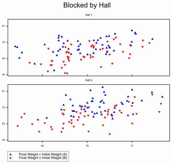
Figure 1 Scatterplot of final versus initial weights of students by hall and diet.
Variant 3
It is now decided to assign students independently to a diet. There is no attempt to block this by hall. (This would be a reasonable strategy if one believed the effect of Hall was negligible.) To what degree numbers are balanced by diet within halls is a matter of chance. As it turns out, the disposition of students is like this.
Count
Diet3 A B
Hall
1 45 55
2 55 45
The code for analysis will look like this.
BLOCKSTRUCTURE Student
COVARIATE Initial
TREATMENTSTRUCTURE Diet3
ANOVA
Here Diet3 is a factor representing how the diet has been allocated.
The output includes the following:
Analysis of variance (adjusted for covariate)
Covariate: Initial Weight
Source of variation d.f.
Student stratum
Diet3 1
Covariate 1
Residual 197
Total 199
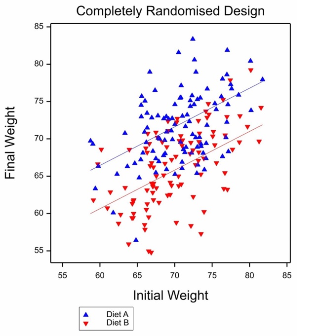
Figure 2 Illustration of ANOVA for a completely randomised design.
How not Why
“However, for statisticians who are trained in “conventional” (i.e. model-blind) methodology and avoid using causal lenses, it is deeply paradoxical that the correct conclusion in one case would be incorrect in another, even though the data look exactly the same.” The Book of Why (3), P217
Well, I am not that straw man and I suspect very few statistician are. I was trained in the Rothamsted approach to statistics and that takes design very seriously and elucidating causes is the central objective of experimental design.
Trialists and medical statisticians will recognise variant 1a as being a cluster randomised design, albeit a rather degenerate example of the class, since there are only two clusters. Variant 2 is a blocked parallel trial, the blocking factor being hall. The clinical trial analogy would be blocking by centre. Variant 3 is a completely randomised parallel group trial. Variant 1b is more unusual. It is theoretical possible and I would not be surprised to find that some clinical trial analogue has been run but I know of no examples.
Each of these four cases leads to a different analysis. It seems intuitively right that they do and John Nelder’s approach delivers a different answer for each.
However, I am not sure that Directed Acyclic Graphs (DAGs) are up to the job. I shall be happy to be proved wrong but must conclude for the moment that it is the causal analysts who will find these four cases deeply paradoxical. They may even refuse to recognise that they are different: if DAGs can’t be drawn to illustrate them, the differences don’t exist.
In fact, it is difficult to decide which of these variants the authors of The Book of Why think they are discussing. Versions 2 and 3 ought to be dismissed from their discussion, yet the proposed analysis that they offer, adjusts the difference in final weights using the within halls regression on initial weights. This is the analysis that is appropriate to variant 3 illustrated in Figure 2. It is very similar to the analysis for variant 1b but the interpretation is different. Variant 1b would not permit separation of Hall and Diet effects.
Wrapping up
Lord’s Paradox illustrates the well-known statistical phenomenon that how data arose is essential to a correct understanding of their analysis. I consider that there are these lessons for causal inference.
- Identifiability is sterile unless it also delivers estimability (8).
- Point estimates are not enough. They are only a small part of the story. Inference must incorporate uncertainty.
- Hierarchical data sets are common, important and require handling appropriately.
- The design of experiments is a powerful field of statistics and is now at least a hundred years old. Although experiments are far from being the only way we make causal inferences, they are an important way that we do. Any causal theory should also be able to handle experiments and learning from statistics will be useful.
References
- Lord FM. A paradox in the interpretation of group comparisons. Psychological Bulletin. 1967;66:304-5.
- Wainer H, Brown LM. Two statistical paradoxes in the interpretation of group differences: Illustrated with medical school admission and licensing data. American Statistician. 2004;58(2):117-23.
- Pearl J, Mackenzie D. The Book of Why: Basic Books; 2018.
- Holland PW, Rubin DB. On Lord’s Paradox. In: Wainer H, Messick S, editors. Principals of Modern Psychological Measurement. Hillsdale, NJ: Lawrence Erlbaum Associates; 1983. p. 3-25.
- Nelder JA. The analysis of randomised experiments with orthogonal block structure I. Block structure and the null analysis of variance. Proceedings of the Royal Society of London. Series A. 1965;283:147-62.
- Nelder JA. The analysis of randomised experiments with orthogonal block structure II. Treatment structure and the general analysis of variance. Proceedings of the Royal Society of London. Series A. 1965;283:163-78.
- Payne R, Tobias R. General balance, combination of information and the analysis of covariance. Scandinavian journal of statistics. 1992:3-23.
- Maclaren OJ, Nicholson R. What can be estimated? Identifiability, estimability, causal inference and ill-posed inverse problems. arXiv preprint arXiv:1904.02826. 2019.
Other related guest posts by Senn include:
Please share your comments.


")


Wonderful post – thank you for yet another impactful post
It poignantly shows how the design is affecting the generalizability of the findings.
Each variant leads to a different generalizability, which is probably how these 4 options should be compared. I mean generalization in the wide sense which is eventually the basis of clinical interpretability, and replicability attempts.
A wide perspective on Lord’s paradox is given in https://en.wikipedia.org/wiki/Lord%27s_paradox
Thanks, for these kind comments Ron. I agree that generalisability is an important issue. However, I think that the generalisability point is somewhat orthogonal to what I discuss here. See the RA Fisher quote on the section on random treatment by block interaction in another blog of mine https://www.linkedin.com/pulse/random-trio-stephen-senn/
Stephen – Fisher did indeed set the seeds for generalizability, The algorithmic methods, based on training-validation splits, add new aspects to this important inferential characteristic. Overfitting implies poor generalizability. The 4 variants you describe lead to different generalizability paths. This relates to how the study outcomes are to be interpreted. In some industries this is framed as a “claim”. It is something that ought to be considered ab initio, if you design an experiment. Head to head are different from comparability studies…
“I shall illustrate the analysis using John Nelder’s approach to designed experiments as incorporated in Genstat®” Whilst I am a great admirer of John Nelder, I am not sure that it is correct to refer to “his approach to designed experiments”. Anyone who learned applied statistics in an agricultural context, as I did, will be all too familiar with nested (or hierarchical) designs, such as the split-plot, in which different levels in the hierarchy have different error terms. The genius of John Nelder, in my opinion, was to make sure that Genstat was fit for purpose when used to analyse a wide range of designs as typically encountered in agricultural research, including hierarchical designs.
In my first five years post university I used Genstat daily. In addition to real work, I managed to find time to simulate data which i would then analyse in Genstat so, for me, it was a tremendous learning tool. When, in 1982, I moved to ICI Agrochemicals i had to make do with SAS. In those days analysis of a hierarchical design in SAS required several different analyses then a hand calculator and a piece of paper.
Another thing I learned in those early years was the importance of clearly identifying the “experimental material” and “experimental unit” in any design. Cox (planning of Experiments, 1958) defines an experimental unit as “corresponding to the smallest division of the experimental material such that any two units may receive different treatments in an experiment”. According to this definition it seems to me that in both Variant 1a and 1b the experimental unit is the hall. So, in both cases we have two halls (units), each receiving a different treatment (diet), and so no scope for carrying out a meaningful analysis. The variation between students is a sub-unit concept of no use in comparing the two diets. In my opinion, the random allocation of students to the two halls in Variant 1b does not change the structure of the experiment when compared with 1a – the treatment (diet) is still applied to the hall (unit), not the student. Now it all depends on how the diets were administered, a detail that we are not given. If 100 students living in 100 houses were allocated at random to one of two diets and had to self-administer the diet, then the experimental unit would be the student – a fully randomised design with no block structure, 100 units and two treatments. But in a hall the students are most likely all eating in a dining room with the diet prepared by catering staff; any misunderstanding or mistake made by the catering staff will then apply to all 50 students on that diet, who are therefore not independent units.
Now, if you are prepared to assume that the hall has no (or little) effect then you can analyse 1b as if it was a fully randomised design, but it is a big assumption. In my career I often came across similar situations in which there was no true replication and was sometimes under pressure to analyse data as if there were. Someone even managed to publish a paper in which sub-unit variation was referred to as pseudo-replication. The fact of publication gave the procedure an undeserved air of respectability.
Peter – The ability of getting differential treatment is indeed a prerequisite to randomization and other study design considerations.
To take this argument one further step, rerandomization is another consideration.
The 1958 book by Cox you referred to is dealing with it – see slides 118-130 in https://ceeds.unimi.it/wp-content/uploads/2020/02/Kenett_Causality_2020.pdf
The reasonable flow seems to be:
1. Determine the goal of the study
2. Map out the generalization requirements of you study
3. Design the study (e.g. variants 1, 2, 3 or 4 …)
4. Conduct the study (was re randomization needed/applied?)
5. Analyze the data
6. Present and generalize findings
Senn is providing important insights by highlighting the importance of what Mayo called “subtle differences”. The challenge is to elevate these differences from the technical domain to the interpretable domain, i.e. the generalization scope of the study.
Currently, these are no good ways to even describe the generalizability of findings.
Senn and Benjamini have focused on treatment block interactions as an impairment to generalizability. I suggest that generalizability needs to be considered in a wider sense…
Peter, thanks for these interesting comments. Elsewhere, I have made it clear that the Rothamsted School was very much more than John Nelder (clearly Fisher & Yates are even more important figures) and conversely one could argue that John Nelder’s approach was more than just the Rothamsted School, since he was not at Rothamsted when he developed it. However, he did formalise the analysis approaches,
I don’t agree that 1a and 1b are the same. It is theoretically possible to consider that what one wishes to study is a combination of unit and treatment. Consider a medical example. In a small town, patients can be treated for a particular condition by Surgeon 1 who uses procedure A and surgeon 2 who uses procedure B. It is decided to run a trial to see which/who is better. There may be no point in trying to separate the effect of surgeon from the effect of procedure and it is an example anyway where the interactive effect could be very important.
Of course, that is a very unusual example but theoretically possible and in creating example 1b I was trying to cover another possibility even if, as ai Made clear in my discussion, it would rarely if ever be of interest.
For those who are interested, there is an extensive online memoir of John Nelder available here https://royalsocietypublishing.org/doi/10.1098/rsbm.2019.0013
I’m very grateful to Stephen for this insightful guest post. I wish Pearl would address the ways these subtle differences in experimental design capture and distinguish types of causal analyses. He seems to assume statistics is inadequate for causal inference.
Thanks, Deborah. As I made clear in the first of my posts on Lord’s Paradox (which you kindly hosted) I consider Pearl’s work to be extremely important. Nelder’s approach is limited to experiments exhibiting ‘general balance’ and of course there are many other forms of investigation we need to make causal inference. Experiments are inherently easier to analyse than observational studies.
Nevertheless, experimental design was extensively studied over the last 100 years and what became clear very early in that study was that there were many traps for the unwary. (Fisher himself fell into one.) These traps do not disappear because one is using observational studies. It is rather that other difficulties appear. So, what I think is that some sort of synthesis of structural causal models and “the Rothamsted School” will be even more powerful.
Note, also, that I reject the excuse that is given for structural causal models of “bias first, then variance”. Part of my argument is that if you don’t understand variances, you don’t know what infinity looks like. See https://errorstatistics.com/2019/03/09/s-senn-to-infinity-and-beyond-how-big-are-your-data-really-guest-post/