

.
Stephen Senn
Consultant Statistician
Edinburgh
Introduction
In a previous post I considered Lord’s paradox from the perspective of the ‘Rothamsted School’ and its approach to the analysis of experiments. I now illustrate this in some detail giving an example.
What I shall do
I have simulated data from an experiment in which two diets have been compared in 20 student halls of residence, each diet having been applied to 10 halls. I shall assume that the halls have been randomly allocated the diet and that in each hall 10 students have been randomly chosen to have their weights recorded at the beginning of the academic year and again at the end.
I shall then compare two approaches to analysing these data and invite the reader to consider which is correct.
I shall then discuss (briefly) what happens to these approaches to analysis when the problem is changed so that we now have not 10 halls with 10 students each per diet but one hall per diet with 100 students each. This is the Lord’s paradox problem (Lord, F. M., 1967) in the form proposed by Wainer and Brown (Wainer, H. & Brown, L. M., 2004). We shall see that one of the philosophies of analysis will indicate that this more difficult case cannot be analysed. The other will produce an analysis that has been previously proposed as the right analysis for Lord’s paradox. I shall then consider what changes are necessary (if any) if we have an observational rather than an experimental set-up.
The data are saved in an Excel workbook here. The first sheet (Experiment_1) gives weights at the beginning and the end of each academic year for each student as well as the hall they were in (numbered 1 to 20); the diet they were given (A or B) and a unique student identification number (1 to 200). The second sheet (Summary_1) consists of mean weights per hall averaged over the students enrolled in the that hall and included in the study.
The approach to analysis
I shall use Genstat’s approach to analysing designed experiments. This is based on John Nelder’s theory of 1965 (Nelder, J. A., 1965a, 1965b) and declares block structure and treatment structure separately. The analyses will only differ as regards the block structure declared, although in one case I can produce an identical analysis using the so-called summary measures approach.
The first analysis
The code looks like this
BLOCKSTRUCTURE Hall/Student
TREATMENTSTRUCTURE Diet
COVARIATE Base
ANOVA [PRINT=aovtable,effects,covariates; FACT=1; FPROB=yes] Weight
The first statement defines the block structure. Students are ‘nested’ within halls. This is written Hall/Student The second states that the (putative) causal factor, the treatment, is Diet. The third declares a covariate, Base, the baseline weight, to be taken account of and the fourth says that the outcome variable is Weight, that is to say the weight at the end of the experiment.
The analysis that is produced is now given in Figure 1.
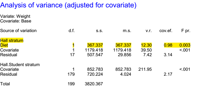
Figure 1 Analysis of the diet data respecting the block structure
I have highlighted the hall stratum and the diet term. Note that there are two residual terms. The first appears in the hall stratum and the second in the students within-halls stratum. Since the diet given is varied between halls but not within, only the former is relevant for judging the effect of diet.
The term v.r. stands for variance ratio. It is the ratio of the mean square (m.s.) for diet (367.3) to the variation term that matters (29.9) the residual for the hall stratum. The ratio is 12.3 so that the analysis tells us that the variation between diets is about 12 times what you would expect given the variation between halls given the same diet.
Note also that there are two covariate terms: both between halls and between students-within-halls. The latter is also irrelevant to any analysis of the effect of diet.
Now consider a second equivalent analysis of this. This just uses the average at baseline and outcome per hall. In other words, it is based on 20 pairs of values (baseline and outcome) not 200. This analysis produces the table in Figure 2. Note that the result is exactly as before, showing the irrelevance of the variances and covariances within halls. That is to say, that although the mean squares change, because now based on averages of 10 students per hall, the ratio of the term for treatment to its residual is the same and so are all inferences. The equivalence of summary measure approaches to more complex models for certain balanced cases is well known (Senn, S. J. et al., 2000).
Note that for both of these equivalent analyses the residual degrees of freedom are 17: there are 20 halls and one degree of freedom has been used for each of grand mean, covariate and treatment, leaving 17. The variation between diets is judged by the variation between halls.
 Figure 2 Summary measures analysis respecting block structure
The second analysis
This uses a different block structure. We now ignore the fact that the students are in different halls. The code becomes
BLOCKSTRUCTURE Student
TREATMENTSTRUCTURE Diet
COVARIATE Base
ANOVA [PRINT=aovtable,effects,covariates; FACT=1; FPROB=yes] Weight
and the output is as given in Figure 3.
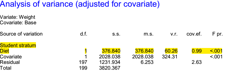 Figure 3 Analysis ignoring the block structure
Note that the residual used to judge the effect of diet is now based on 197 degrees of freedom and it is less than a quarter of what it was before (6.3 as opposed to 29.9). The numerator of the variance ratio is somewhat similar to what it was before (a different covariate term has been used to adjust it so there is some difference) but the variance ratio is now five times what it was. The result is much more impressive.
Which analysis is right?
A long tradition says that the first analysis is right and the second is wrong. In a clinical context, the experiment has a cluster randomised form. The regulators, the EMA and the FDA, will not let drug sponsors analyse cluster randomised trials as if they were parallel group trials but this is what the second analysis will do.
“No causality in, no causality out” is a common slogan but the actual intervention here did not take place independently at the level of students but at the level of halls. It is this variation (between halls) that should be used to judge treatment. Speaking practically, the halls may be situated at different distances from lecture theatres on campus so that exercise effects may be different. Some may be closer to food shops and so forth. One can imagine many effects independent of the diet offered that would vary at the level of hall but not at the level of students within halls.
But isn’t this a red-herring?
I have considered a randomised experiment involving many halls. It differs from the situation of the paradox in two respects. First, there were only two halls and second the diet was not randomised. We can summarise these differences as ’two not many’ and ‘observational not experimental’. I consider these in turn.
Two not many
There are only two halls in the Lord’s paradox case. This means that analysis one is impossible and only two is possible, which is an analysis that has been previously proposed as being right for Lord’s paradox. You cannot estimate the relevant variances and covariances for approach one if you only have two halls. (See my original blog on the subject.) I have no objection to analysts defending approach two on the grounds that this is all that can be done if an analysis is to be done. In fact, I have even given this analysis some (lukewarm) support in the past (Senn, S. J., 2006). However, two points are important. First, it should be recognised that a third choice is being overlooked: that of saying that the data are simply too ambiguous to offer any analysis. Second, it should be made explicit that the analysis is valid on the assumption that there are no between hall variance and covariance elements above those seen within. It should be made clear that this is a strong but untestable assumption.
Observational not experimental
I can think of no valid reason why analysis two could become valid for an observational set-up if it was not valid for the experimental one. I can imagine the reverse being the case but to claim that an invalid analysis of an experiment would suddenly become valid if only it had not been randomised despite the fact that no different or further data of any kind were available, strikes me as being a very unpromising line of defence. Thus, I consider this the real red herring.
Does it make a difference?
In this case the between halls regression is very similar to the within halls regression: the slope in the first case is 0.57 and in the second is 0.55. Furthermore, the means at baseline for the two diets are also very similar; 75.1kg and 76.1kg. This means that the estimates of the diet effects (B compared to A) are nearly identical 2.7kg versus 2.8kg. The situation is illustrated in Figure 4, the estimated treatment effect being the difference between the corresponding pair of parallel lines.
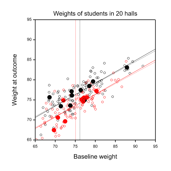 Figure 4 Two analyses of covariance. Red = Diet A, Black = Diet B. Open circles and dashed sloping lines, students. Closed circles and solid sloping lines, halls. Vertical dashed lines indicate mean weights per diet at baseline.
It might be concluded that the distinction is irrelevant. Such a conclusion would be false. Even in this case, where estimates do not differ, the standard errors of the estimates are radically different. For the between-halls analysis the standard error is 0.78kg. For the within-halls analysis it is 0.36kg. The relative evidential weight of the two, say for updating a prior distribution to a posterior for any Bayesian, or for combining with other evidence in any meta-analysis, is the ratio of the square of the reciprocal of the standard errors, that is to say 4.7. The analysis based on students rather than halls overstates the evidence considerably.
In summary
I maintain that thinking carefully about block-structure and treatment structure as John Nelder taught us to do is the right way to think about experiments. I also think, mutatis mutandi, that it can help in thinking about some causal questions in an observational set-up. Variation can occur at many levels and this is as true of observational studies as it is of experimental ones. In making this claim it is not my intention to detract from other powerful approaches. It can be helpful to have many tools to attack such problems.
References
Lord, F. M. (1967). A paradox in the interpretation of group comparisons. Psychological Bulletin, 66, 304-305
Nelder, J. A. (1965a). The analysis of randomised experiments with orthogonal block structure I. Block structure and the null analysis of variance. Proceedings of the Royal Society of London. Series A, 283, 147-162
Nelder, J. A. (1965b). The analysis of randomised experiments with orthogonal block structure II. Treatment structure and the general analysis of variance. Proceedings of the Royal Society of London. Series A, 283, 163-178
Senn, S. J. (2006). Change from baseline and analysis of covariance revisited. Statistics in Medicine, 25(24), 4334–4344
Senn, S. J., Stevens, L., & Chaturvedi, N. (2000). Repeated measures in clinical trials: simple strategies for analysis using summary measures. Statistics in Medicine, 19(6), 861-877
Wainer, H., & Brown, L. M. (2004). Two statistical paradoxes in the interpretation of group differences: Illustrated with medical school admission and licensing data. American Statistician, 58(2), 117-123


")


Stephen: Thank you so much for the follow-up guest post!
Lord paradox is a causal problem. In the story, each statistician proposes a method of estimating the causal effect of diet on weight gain. To discuss the notion of “valid” as it relates to “causal effect” we must invoke causal vocabulary. We cannot do it in the vocabulary of variances and covariances no matter how intricate.
It is for this reason that I find myself unable to relate Stephen Senn’s post to the original paradox posed by F. Lord. Nor can I related it to my analysis of the Lord paradox in the Book of Why http://bayes.cs.ucla.edu/WHY/
As a student of paradoxes I would need the following information to get started:
1. What did the statisticians attempt to estimate in the non-experimental case.
2. My analysis ignores completely the Rothamsted School and Nedler’s analysis. What part of the analysis would improve by attending these sources.
3. We know that any exercise in causal analysis must rest on some untestable causal assumptions. What are the assumption that Senn wishes us to consider in the non-experimental case,
4. We know that causal assumptions cannot be expressed in the language of statistics. What language
does Senn prefer for expressing those assumptions.?
5. Senn argues that his analysis “can help in thinking about some causal questions”. We are fortunate to live in an era where we no longer need such help. Causal inference permit us to formulate things mathematically and derive answers to causal questions, rather than “thinking” about them.
To answer your questions
1) The research question is “what is the effect of diet on weight?”.
2) What is missing is a) an explanation as to what conditioning on /adjusting for the baseline weight means (there are at least two possible approaches) b) an explanation as to how the standard error would be calculated.
3) If causal analysis cannot provide standard errors you cannot weight evidence. So much the worse for causal analysis. Suppose two scientists had investigated the same causal question in different studies coming to slightly different answers. How do you propose to combine the evidence?
4) Please provide the valid reason as to why one of the two answers I gave rather than the other is correct. I gave an answer.
5) Do you have a theory of the strength of evidence? John Nelder’s approach provides an answer.
In connection with the latter, I have three questions for you.
1) Can the causal calculus analyse designed experiments?
2) If so, how are the following three cases analysed? In all cases two different training programmes for students are being compared to determine the effect on weight. In all three cases the students are drawn from two halls and in all three cases the length of follow up is the same-
i) The design is blocked by hall. One hundred students in each hall are randomly assigned to one of the two programmes, 50 students per programme per hall.
ii) The design is confounded with hall. One of the halls is chosen at random and 100 students in that hall receive one programme and 100 students in the other hall receive the other programme.
iii) The design is completely randomised. This leads to some students in each hall being allocated to one programme and some to another but with no guarantee that there will 50 students on each. By the time it comes to analysis it has been lost as to which student was in which hall although the other data are available.
Standard statistical theory says that these three experiments provide different amounts of evidence, despite the fact that each involves 200 students. The first is the most precise and the second the least , with the third being somewhere in between the two. John Nelder’s approach, incorporated in Genstat, explains how to analyse such experiments and would award the results different standard errors. Actually, for experiment ii) no standard error can be calculated.
This leads to my third question.
3) Is it the case that in causal analysis all studies are equal? Or is there any way in which one can assess the relative claims of different estimates (each of which has been declared OK by the causal calculus)?
“Actually, for experiment ii) no standard error can be calculated.” Shouldn’t we add to that “without further assumptions”? I ask because it seems if I assume each hall to have a fixed outcome under one treatment with assignment to the other group producing only a fixed shift d to that hall’s outcome, it seems I can calculate a standard deviation for hall difference over the equiprobable two-point sample space created by the randomization of the two halls. What am I missing?
Sander, I suppose you can answer anything given enough assumptions. It is not entirely clear to me what you are proposing Can you demonstrate what the answer is if we only have Halls 1 and 11? Here are the data
Diet Hall Student Baseline Weight
A 1 1 72.13505716 72.78108306
A 1 2 72.06549128 69.46830602
A 1 3 73.7651869 70.69768912
A 1 4 65.24198484 65.12219917
A 1 5 70.01472376 71.79846577
A 1 6 69.30490781 72.66325177
A 1 7 75.49516229 73.24678327
A 1 8 69.21354263 70.52437937
A 1 9 70.33087372 68.82745824
A 1 10 69.04869264 70.79664556
B 11 101 76.35978996 77.07327479
B 11 102 73.85362621 72.26753361
B 11 103 75.59114477 78.57814668
B 11 104 80.68426934 80.54510497
B 11 105 89.3258647 84.58584333
B 11 106 72.33999088 77.19185567
B 11 107 77.79337407 78.18646521
B 11 108 87.32350464 83.5651827
B 11 109 82.3035174 81.76323258
B 11 110 78.81909101 82.22546732
Thanks. Stephen
PS My apologies about the ridiculous precision in the numbers.
“I suppose you can answer anything given enough assumptions.” Yes but you can’t answer anything without assumptions. Randomization is always a huge assumption (the biggest one in causal analyses), assuming that someone did something very physical (force treatments on the units based on a randomizer within levels of any blocking factors); it’s really a set of assumptions whose number corresponds the residual degrees of freedom for the propensity-score regression. Randomization claims are often taken for granted in discussions of the “replication crisis” but shouldn’t go unquestioned in clinical trials.
To answer your question let me simplify to hall with A: mean baseline x_bar=70, mean outcome y_bar=72, hall with B: x_bar = 74, y_bar 75. Let Z be the indicator for treatment A. Assume the individual-level structural model
y = x + b*z + e where e is a mean-zero error independent of hall, individual, x, and z.
Then I presume this model gives us the estimate b_hat = (72-70)-(75-74) = 1 with error variance var(e) found by pooling the variances of y-x from within the halls, giving us a standard error for b_hat.
Of course this example might be mistaken, but still the availability of a standard error (or any estimate for that matter) depends entirely on what you assume; if it’s not identified under your model it is instructive to see what extra assumptions (constraints) will identify it. Those additions are never unique, and some may be plausible.
More generally (and I suspect you as well as both Mayo and Judea could comment well on this), I think it helpful to emphasize that “statistical inference” as ordinarily taught is just a collection of deductive forms. Then the fact that the givens don’t identify a quantity is not too alarming if additional plausible working assumption would do so – especially knowing that all identification is purchased with assumptions.
None of that undermines your thematic points, but I conjecture that Judea is accustomed to injecting qualitative identifying assumptions via the classically unfamiliar route of introducing a formal causal model (although of example of statisticians doing exactly this date back to the 1920-1930s). An argument for doing so is that the plausibility of the additional assumptions is much more easy to evaluate for the subject-matter expert, given their causal-mechanistic form (“no effect”) instead of a probabilistic-associational form (“statistically independent”); I think this is why some writers refer to the causal diagrams which encode these assumptions as “Bayes nets”, the “Bayes” in deference to the fact that those assumptions are contextually-based prior information. I have argued that there are deep hazards in doing so (Greenland S, 2010, “Overthrowing the tyranny of null hypotheses hidden in causal diagrams.” Ch. 22 in: Dechter et al., “Heuristics, Probabilities, and Causality: A Tribute to Judea Pearl.” p. 365-382), reflecting the usual objection that the experts can be too uncritical of their own nulls; but as with all deductive exercises it is still useful if not taken as “revealing truth,” as witnessed by the sizeable literature on using causal models to account for randomization failures such as nonrandom nonadherence and drop-out.
Here is an alternative analysis.
The first step is to look at the boxplots (i) of the initial weights and
(ii) of the changes in weights. These are plotted in such a manner as
to be able to relate one to the other. When writing a paper on the
data the boxplots should be shown.
The boxplots (i) show that Hall 19 is a large outlier with initial
weights of the order of 85kg. This is associated with decreases in
weight of the order of 5kg, the largest decrease being 8kg. Hall 15 is
exotic in the boxplots (i) but is clearly an outlier in the
boxplots (ii). Hall 15 is the opposite of hall 19. The initial weights
are of the order of 70kg and these are accompanied with increases in
weight of between 3kg and 11kg. The weight of lightest student
increased from 60kg to 71kg. Both Halls were on the same diet. This is
remarkable. The data should be checked for accuracy. If they are
correct an explanation should be given for the large differences in
weights of the students from the two halls. I find it difficult to
give a convincing story. Assuming a convincing story is found can this
also explain the different effects of the diet? This will be an
important part of any paper.
A next step could be to look at halls with similar initial
weights. Halls 1, 5, 13 and 15 have initial weights of about
70kg. Plotting these against the changes in weights show that there is
a decrease in weights in Halls 1 and 5 on diet A . For the Halls 13
and 15 on diet B there is an increase in weight.
Halls 2, 3, 4, 6 10, 11, 12, 17 and 18 have similar initial
weights. Plot shown that there is an almost linear increase in weight
loss for all halls apart from hall 18. The data of Hall 17
have one outlier which will effect the result of any linear
regression. Hall 3 has 3 extreme points which again will influence the
result of any regression. In general the weight losses are less for
Diet B.
In site of the presence of outlying observations in some halls I now
regress the change in weight on the initial weight for each hall
separately and plot the slope as a function of the offset. The result
is almost a straight line. The intercept and slopes are
diet A
(Intercept) 0.0084378
slope -0.0141432
diet B
(Intercept) 0.022928
slope -0.013426
There are three exotic values, the Halls 7 13 and 18 which have small
slopes. Hall 13 has the smallest slope -0.010. This negative
slope is due to one outlier with initial weight 80kg. If this
is removed the slope is now +0.097 making Hall 13 even more of an
outlier so to speak.
And so on.
Thanks, Laurie, for taking the time to look at the data in detail. There are, however, a number of points in this analysis that I would query but in particular that it does not really address the block structure apart from an exploratory analysis (the various box plots) which does, at least, look at things hall by hall. Secondly, I object to regressing change in weight. Why? Causes do not require change. For example, if a beauty cream led to individuals who took it having no change in looks over twenty years, it would clearly have had a dramatic effect. The correct standard is the counterfactual ‘what would have happened’ not the state at the start of the experiment. This is only ever adequate as an approximation to what would have happened but in a controlled experiment it is the control group that tells. The past is not on offer. In fact, as Nan Laird has shown, if the baseline is included as a covariate, it makes no difference whether you use the change score or the raw outcome. Personally I prefer not to analyse changes from baseline.
Thirdly, you appear to use what happens within halls to judge which are outliers. However the correct regression only needs the mean values by hall. Whatever happens to the individual students within halls that is of relevance to the causal inference is summarised by the average values for the halls as a whole. It is the variability between halls that is important here, not within, and your analysis as a whole concentrates far too much on the latter. In any case, neither for final nor for baseline weight does Bartlett’s test give any grounds for any believing in systematic (as opposed to random) variation in variances from hall to hall, nor, when one uses mean values per hall, from diet to diet.
Reference
1. Laird NM. Further comparative analyses of pre-test post-test research designs. The American Statistician. 1983;37:329-330.
A key feature in Lord’s paradox is that the groups are noticeably different at the beginning. This doesn’t seem to be the case in the simulated experiment. If the data generation process doesn’t model any correlation between baseline weight and diet, is it really relevant to the discussion?
The “additional assumption” in Pearl’s argument is that “the initial weight is the only variable that can conceivably affect both the final weight and the choice of diet”. The main point is that a causal model is needed (and I agree, even though I find that causal link somewhat unrealistic [*]).
Considering that the initial weight and the diet are independent is also an implicit “additional assumption”. And if the data shows a strong correlation between initial weight and diet, that assumption may be suspect.
[*] As stated in the “Kumbaya” paper, “[the initial weight] is in fact a confounder since, as shown in the data, overweight students seem more inclined to choose Dining Room B, compared with underweight students. So, WI affects both diet D and final weight W.”
If the choice of dining room (and therefore diet) depends only on the initial weight WI, the link is “WI -> D” (and W depends on both) so we have to control for WI get the causal effect of D on W.
But it’s reasonable to think that there is some common cause (like gender or lifestyle) of initial weight and dining room / diet choice (maybe in addition to the direct link). Controlling for WI could be still enough if the common cause Z doesn’t have a direct effect on the final weight. But if there is a direct link one would have to control for Z (maybe in addition to controlling for WI).
Some points in reply.
1) First of all, the experimental set-up I described is much better behaved than Lord’s paradox. Note, however, that I am claiming that even in this better behaved case the solution that has been proposed for Lord’s paradox does not work without assumptions that need to be made explicit. If I had been proposing the reverse. If for example, I had said ‘what s all the fuss about? I can show you how you can validly analyse a randomised experiment’, then the criticism would be valid. However, that is not what was said. I said, ‘even if the experiment were randomised, this would not work’. Unless an argument can be produced to show that an analysis that is invalid for a randomised experiment would work for one that is not, your criticism beside the point.
2) The example does have correlation between baseline and outcome. It was simulated to have two correlations, one between hall and one within. I set the former to 0.5 and the latter to 0.7 in the simulation. In fact, the crude observed correlation of the per hall means (ignoring diet) is 0.47 in the data and the overall correlation (ignoring hall and diet) is 0.68
3) Note that it is easy to produce a non-randomised experiment with strong differences between baseline weights per diet group in which analysis of covariance using within-hall covariances would be (plausibly) valid. This is to employ a so-called regression discontinuity design. We choose one hall only. In that hall we ask a number of students to participate in a study and weight them. The heaviest half (those above median weight) are given an intervention designed to affect weight and the other half (those below the median) are taken as a control group. This does not require any assumption about between halls variance and covariances being the same as within hall covariance and variances because the intervention is only varied according to the baseline weight of the student and not according to the hall the student is in. It does require an assumption that the relationship between baseline and outcome is linear over the range studied.
Thus, as I have maintained all along, the key to understanding this is to look at the block structure, which is Hall/Student and not Student.
We agree that your example is well-behaved (there is no paradox, because the argument “John uses a so-called change-score […] John thus concludes that there is no effect of diet on weight.” doesn’t work here). It’s also different from the original problem in that it has students nested within halls, and this extra complexity obviously requires additional assumptions.
In the original problem, the causal link “WI -> D” does actually have an intermediate step “WI -> H -> D”. If the only influence of the hall on the outcome is through the diet, it doesn’t matter. If the hall has a direct effect on the outcome (and as you said “one can imagine many effects independent of the diet offered that would vary at the level of hall but not at the level of students within halls”) then it does matter.
But there is nothing that can be done about it. There is no way to control for H when it has a one-to-one correspondence to D. In fact we don’t compare the effects of Diet A and Diet B. We compare the effects of Diet A in Hall 1 with Diet B in Hall 2.
In your example, you present two analysis and argue that “the analysis based on students rather than halls overstates the evidence considerably”. Of course that’s only true if there is actually a direct effect of the hall on the outcome (which I agree is a reasonable assumption to make).
Note that causal analysis will tell you the same thing: if there is a direct effect of the hall on the final weight (not just through “H -> D -> W”) you have to control for H. By the way, that would also take care of the eventual confounders Z that I mentioned in my previous reply (if there was a causal relation “WI H -> W” with Z being also a direct cause of W).
Thanks. Your comments are helpful. However, one clarification, although the original example talks about girls and boys, I was considering the Wainer and Brown version, which is the version discussed in The Book of Why. However, I suppose that if one takes the point of view what is the combined effect of diet and hall? then one could ignore the hall effect and no longer treat it as a block but instead it could become part of the treatment. For example, one could consider the causal questions to be: “what happens to weight if a student is assigned to eat in hall 1 (currently using diet A) rather than hall 11 (currently using diet B)?”, rather than, “what happens if the diet in halls in general is switched from A to B?”. In the first of these two the block structure is just student but block and hall are confounded treatment effects. In the second hall becomes part of the block structure.
More generally, however, I am puzzled as to how random effects are incorporated. In a sense, since students are also causal agents, they are also part of the diagram but if each student is added the whole thing becomes hopeless. The usual way that statisticians deal with explosion of parameters is to treat them as random and thus replace them with a distribution. What statisticians (and other researchers) realised in agriculture a long time ago, however, is that such variation can occur at many levels. It is dealing with this feature that is a key strength of John Nelder’s approach.
Great explication.
It makes me wonder – when there two halls us it better to throw away the data from one hall?
Better in the sense of at least getting a clean estimate of the change.
There “only” was an exploratory analysis. The word change was and is meant in a purely neutral sense, change, difference, increase decrease, it’s all the same to me. I made no use of any concept of cause, a concept I am somewhat suspicious about. The best book I know on data analysis is by Peter Huber, Data Analysis: What can be learned from the past 50 years. The word cause is never mentioned. I also wrote a book on data analysis, Data Analysis and Approximate Models, again no causes. You could have told me a different story, the EDA woul have been the same.
The boxplots show that Halls 15 and 19 are outliers or, if you prefer, exotic in the sense of Tukey. No concept of causality is required for this observation. In an ideal situation the statistician would analyse the data together with the person who collected it. You have provided a story so my first question would by why do Halls 15 and 19 differ so much. Do they choose their students by weight? One possibility is that Hall 15 is well known for its frugality, a single hard bodied egg for breakfast, 1000 calories a day. Hall 19 are the gluttons, a full English breakfast followed by two glasses of wine in preparation for the day o come, 2000 calories per day. The diet is 1500 calories per day which would sort of explain the results. Halls 21 and 22 were not included so here the counterfactuals. Hall 21 chooses long distance runners with weights similar to those of Hall 15. They have a diet of 2000 calories and their weights are kept low by their training. Hall 22 consists of people with weights similar to those of Hall 19 but who are overweight for some medical reason. They have a special 1000 calory diet. If both Halls were put on Diet B those in Hall 21 would lose weight, those in Hall 22 would gain.
“Thirdly, you appear to use what happens within halls to judge which are outliers. However the correct regression only needs the mean values by hall. Whatever happens to the individual students within halls that is of relevance to the causal inference is summarized by the average values for the halls as a whole.”
I didn’t realize that there was such a thing as a “correct” regression. What I am doing is to point out differences between the Halls. Halls 13,16 and 18 show only small trends. Halls 12, 14 and 17 show strong trends. Their baselines are similar. You say, ‘irrelevant’, the person who collected the data says ‘that’s interesting, I wonder why. I will go and check the data’.
Suppose in every hall I now alter the second measurement so it is an exact linear function of the first with positive slope but with the same mean and variance as the actual data. If your analysis depends just on means and variances you would come to exactly the same conclusion, a sort of Simpson’s paradox, every where a strong positive relationship but overall nothing to report.
The main points of interest are (i) how do the Halls select their students and (ii) the exotic Halls 15 and 19. Your analysis gives no hint of the latter.
You make a very good point here, Laurie, and it’s one that should be taken on board by all analysts: there is more to know than just the numbers. I like to remind my students that the scientists knows more about the system under study than the statistics do. The intricacies and convolutions of a sophisticated statistical analysis can blind the analyst to relevant real-world considerations at same time as it makes clear patterns and relationships within the numbers.
A child sees an ice cream parlour on the opposite side of the road. The pedestrian traffic light is green, he runs across to buy an ice-cream and is hit by a car whose driver was texting. What caused the accident?
do(no ice-cream parlour)
do(no money)
do(do no texting)
do(pedestrian traffic light red)
do(road traffic education: look right, look left, look right again and if all clear cross the road)
If we wish to take some action to prevent such accidents in future we will have to “think” about the causes, as will the judge.
They all caused the accident. Every event has innumerable causes; the questions of interest ask which ones are measurable, relevant (e.g., morally), modifiable, etc. and are clearly context dependent.
The issue of modeling multiple causes is taken up in many places, e.g., under the topic of sufficient-cause models, an introduction to which can be found in Ch. 2 of Modern Epidemiology (Rothman et al., 3rd ed. 2008) with much more detail worked out since in many articles by Tyler VanderWeele (see also his book, Explanation in Causal Inference, 2015).
Sander, exactly. It seems to me that you can always find multiple explanations if the groups under consideration are not homogeneous, different explanations for different groups. The EDA made it clear that the Halls are not homogeneous so end of story. This seems to be the explanation of Lord’s paradox. Huber mentions only heterogeneity when discussing Simpson’s paradox, no mention of causality. And even if they are homogenous you can probably find multiple explanations as above. At this level I fail to see how a calculus of causality can help.
“At this level I fail to see how a calculus of causality can help.”
“At this level” is unclear to me; what level?
Heterogeneity isn’t the end of the story, it should be at the start as it is almost omnipresent – there are few practical examples in health and risk assessment for which homogeneity is remotely plausible and I suspect the same is true for education and social science. Does that imply causal models using the assumption are useless? Far from it! Such models are often quite adequate for estimating effects on population means. And if needed they can be extended to include any degree of heterogeneity one wishes, to identify and estimate major sources of heterogeneity.
There is a lot of statistical developments that explain all that, albeit not in Pearl’s work (which focuses on causal theory, not its integration into statistical inference) or in Modern Epidemiology (beyond very brief description and reference in the 3rd ed.), but it can be seen in articles on g-estimation, marginal structural modeling, and doubly robust estimation – including methods for mediation and interaction analysis (e.g., in VanderWeele’s book). Your comments seem to overlook all these recent developments; if am mistaken I would like to understand how you can make such a dismissive and in my view incorrect “end of story” comment, for one could build these models into this example, and they have been applied to far more complex ones.
As far as I can tell the whole Nelder-theory aspect of focus here is only about what block-randomization assumptions do or do not identify statistically (such as a standard error to attach to a point estimate); but, as in my earlier toy-model in response to Senn, one can go on to specify causal models that do provide such identification, and those can be as multifactorial as needed although for most very real problems only one or maybe two factors are key. In your example, all the court will judge by is that the pedestrian had the right of way – judgment thus goes against the driver. No model needed for that; however an accident researcher may include (along with light status) texting as a key variable for policy (law) formulation, and thus use a causal model with both to estimate the population impact of anti-texting laws.
Yes I do overlook it for the simple reason that I have not read any of it. I have just read Pearl on Lord’s paradox and it comes down to the fact that some girls have weights not represented by the boys and vice versa. So you have no evidence on how the diet will effect boys with low weights because you have no data there. Similarly for girls with large ones. End of story in “The EDA made it clear that the Halls are not homogeneous” and I have not read anything on Senn’s example which would cause me to alter this opinion. Senn suggests just comparing Halls 1 and 11. Seems very odd to me, their x-supports are almost disjoint. Hall 1 shows a strong decrease of final weight as a function of initial weight as does Hall11. Plot them together it disappears. Both you and Senn use means and don’t mention the depedency. As we are interested in the effect of diet on weight this strikes me as odd.
Fair enough about Senn’s numbers and the oddity in the discussion. My focus was however to place his general point (about randomization-based inference) more clearly in the language of causal modeling, which is what Judea speaks in, and point out how formal causal assumptions can be combined with traditional statistical ones to show where we may get identification. I did not and do not care about the particular numbers. Maybe this will explain why:
The nonoverlap problem you focus on is widely discussed in the causal modeling literature and dealt with under the assumption of “positivity” (the assumption that there are no zeros (or no near-zero probabilities, for theorems) in the covariate-specific treatment distributions. Postivity is often misrepresented as a general necessary condition for causal inference but that is incorrect; it is only necessary for certain methods that do not smooth out zeros or undefined 0/0 ratios. As you said, it would be “end of story” for those methods and I think common intuition goes to that place and stays there. That’s playing safe; other methods however replace those quantities with model-based expectations, which may be innocuous interpolations (e.g., between a 15 and 20 mg dose) or perilous extrapolations (e.g., hormone effects across sexes).
It’s very context dependent and controversial as to innocuous vs. perilous. But once we recognize that everything is riding on assumptions, it is wrong to say “you have no evidence on how the diet will [affect] boys with low weights because you have no data there.” Not quite: If you assume that to some extent the diet effects are similar across sexes (as for example high-carb vs high-fat diets – that literature emphasizes the extensive metabolic similarities across sexes along this axis) then you can extrapolate between them based on (for example) a prior for the sex-shared effect and data from one sex becomes evidence for the other (with some discounting). Do statisticians do this? Yes: In frequentist theory it’s called “borrowing strength” and seen in the empirical-Bayes literature; the Bayesian version is based on the same structural model with the usual difference in probability interpretation (bets rather than sampling frequencies).
(Apologies if all that misses your concern.)
One clarification. My examination of the basic structure of the problem lead me to claim that any analysis of a problem based on two halls only would be problematic if diet was varied at the level of hall only (and not at the level of students with halls). I did not expect analysis of the two hall problem to come to any reasonable conclusion. I simply posted the example with two halls only (from the original 20 in my simulation) so that anybody who disagreed could post their analysis.
Actually, I think that the 20 halls example is better for promoting understanding but I was criticised as having unfairly changed the example so posted the two halls example for those who wished to deal with it.
In correspondence with Stephen I came to realize that I was unclear in describing my toy-model example, in which identification was achieved by leaving out block effects. With apologies for that, I would combine and expand my remarks to both Stephen and Laurie as follows:
By assuming block effects were zero we have no confounding. Suppose now we drop this obviously mistaken assumption by expanding the individual-level structural model for the two halls with an indicator h for hall, as
y = x + b*z + c*h + e where again e is a mean-zero error independent hall h, individual, x, and z. With only two halls, h and z are perfectly associated and so treatment and hall effects are completely confounded, hence we get no identification of the treatment effect without further constraints.
A Bayesian could identify the treatment effect b by putting a prior on the hall effect c, which could be described as treating c as a random coefficient with known mean and variance (and which could be based on literature on gender effects if the difference between halls was solely in their gender difference); the prior on the treatment effect could be left improper if desired (making this analysis partially Bayes in the sense of Cox 1975 in using a prior for nuisance parameters only). Meanwhile a frequentist could identify b by fixing c at a value c0 and fitting the offset regression
y = x + b*z + c0*h + e, repeating this for various c0 in a sensitivity analysis (the range of variation could be based on literature on sex effects if the difference between halls was solely in their sex difference); in effect this is like repeating a partial-Bayesian analysis with different point-mass priors on c.
The perhaps obvious and tangential point of this belaboring is that it is inaccurate (and I think potentially misleading) to say an effect isn’t (or is) identified, or we can’t (or can) get a standard error, or we have run out of degrees of freedom, or there is uncontrollable confounding, or “end of story” or whatever terminating claim without conditioning that claim on “given the assumptions we have made” or “under the given model” or something like that. There is always a way to extract information from data about our target effect using further assumptions (e.g., the block effect is c0) to process the data information (e.g., that the blocks don’t overlap on gender). Ideally these assumptions are based on valid external information, like how gender affects outcome (I regard a nondegenerate prior as an assumption, albeit a fuzzy one) but often they are just simplifying conveniences we hope are innocuous (like additivity).
Again, I think that all we are ever doing with statistical procedures is using assumption sets (models) to extract data information. What matters is whether the stakeholders in the problem accept the model and thus are forced to accept the deductions from it and the data (or not). Apologies for belaboring this point , which might seem too obvious or off-topic here. But it also seems to me that the family of examples discussed under “Lord’s paradox” and Senn’s comments can be most easily framed in these terms by adding in a causal-model layer as Pearl wants. And that furthermore, identification flexibility and credibility can be greatly enhanced by using fuzzy assumptions (soft constraints), such as those encoded by penalty functions or priors. We should thus keep these options in mind when confronted with real problems resembling the examples.
Any corrections, exceptions, or extensions will be appreciated.
I did not suggest just comparing hall 1 and 11. I reduced the 20 halls example to just 2 halls so that any analysis anybody had could be exhibited on this.I regards the 20 hall case as being more interesting because here two alternative analyses are feasible. One of these is still feasible in the two hall case. However, I would not use it in the 20 hall case and this should, at least, give pause for thought. As regards residuals, bear in mind that for the analysis I regard as correct, there are only 20 residuals. Here http://www.senns.demon.co.uk/ANCOCA%20mean%20weights.jpg is a plot of them. I don’t regard this as being particularly worrying. However, even if i do plot the data at the student level, I don’t find this particularly peculiar. Here is a trellis plot http://www.senns.demon.co.uk/Lords_Trellis.jpg
The estimate, for this analysis is 2.61 kg with a standard error of 1.21 kg on 17 degrees of freedom and (at the risk of offending the great and the good) a P-value of 0.046, which I shall describe as a trend towards non-significance but then, there is quite a lot of variation between halls and rather few halls.
Of course, I have an unfair advantage over everybody else, in that I am the god of this simulation universe and set the diet effect to be 3 kg.
But, I should stress also, that although in practice, data-examination is an important part of any analysis, my objective here was to look at the paradox through design of experiments spectacles rather than exploratory data-analysis ones.
The ‘end of story’ was too lazy. It’s easy to criticize, harder to do something positive. So here is my analysis of the data.
Denote the initial weight by x_i and the final change in weight by y_i. We try and approximate the y_i by a simple function f of x_i, y_i=f(x_i). Can this be done with the same function for all the 200 data points? A linear regression shows that this cannot be done. For f linear, the residuals for Halls 1-10 are mostly negative and those for Halls 11-20 mostly positive. A little thought shows that there is no monotone function which will give a reasonable approximation. Any function which achieves this will have a large number of local extreme. Can the Halls 1-10 be approximated by the same function. A linear regression shows that this is not possible for as Halls 5 and 9 cannot be so approximated and require their own regression function. Similarly halls 11-20 cannot be approximated by a common
linear function.
This leads to approximating the data in each hall by a different function f. The simplest function is the constant which we take to be the mean. As a measure of approximation I take the number of changes in sign of the residuals. These are
1 1 1 3 3 3 3 3 3 3 3 3 4 4 5 5 5 6 7 7
Simulations show that the probability of at most three changes in sign for samples of size 10 is about 0.2. Using this I get a P-value of 1.516284e-05 for the above sequence. In other words reducing the
individual halls to their means means ignoring the structure that the data have. One can do this but at least it should be pointed out that this is so. It also seems strange to ignore the structure as this is
the point of the whole exercise.
So as simple means don’t work we can try a linear regression for each hall. The number of changes in sign for the twenty halls are now
3 4 4 4 4 4 5 5 5 5 5 5 6 6 6 6 6 6 7 7
This works, each hall can be approximated by a linear regression but what now? I am not sure. You can plot the intersections and slopes against the mean of the x_i for all twenty halls, the mean of the x_i being a proxy for the support of the ith hall. If you do this you see that there is not much difference between the halls except for halls 13,18 and 19. Hall 19 does not have exotic values for either the intercept of the slope, it is just that its support is a long way off. There is no systematic difference between the halls 1-10 and 11-20 minus the exotic ones. What this has to do with causality is another matter.
I was also talking about the Wainer and Brown version… or so I thought until I read their description.
They “misquote” Lord’s problem, suppressing the fragment in brackets: “A large university is interested in investigating the effects on the students of the diet provided in the university dining halls [and any sex difference in these effects.] Various types of data are gathered. In particular, the weight of each student at the time of his arrival in September and his weight the following June are recorded.”
In the original problem, there are an unspecified number of dining halls and all of them serve the same diet. The question is whether the “effect” of the “treatment” (there is no “control”) is different in the subgroups “girls” and “boys”. Wainer and Brown call the subgroups “Dining Room A” and “Dining Room B” but there is still one single diet: the “treatment”. The only mention of “diet” in their description is to say that the results of the first and second statisticians corresponds to different assumptions about the effect of the “student’s control diet (whatever that might be)”.
In the discussion of how the model can be applied to the medical school data they say: “This layout makes clear that the control condition was undefined – no one was exposed to C (S=T for all students) – and so any causal analysis must make untestable assumptions. As is perhaps obvious now, the two different answers that we got to the same question must have meant that we made two different untestable assumptions.”
They don’t mention why do they change the problem to have subgroups in terms of dining rooms instead of sex. They don’t explain why the characteristics of the students in each dining room are different. They don’t discuss what could be the cause for a differential effect of dining room.
It is not an alternative to the original one, it’s a generalization. If all the boys go to dining room A and all the girls go to dining room B we recover Lord’s formulation.
Pearl says in the book “A 2006 paper [*] by Howard Wainer and Lisa Brown attempts to remedy this defect. They change the story so that the quantity of interest is the effect of diet (not gender) on weight gain, while gender differences are not considered. In their version, the students eat in one of two dining halls with different diets. Accordingly, the two ellipses of Figure 6.7 represent two dining halls, each serving a different diet (…) Lord’s paradox now surfaces with great clarity, since the query is well defined as the effect of diet on gain.”
I think the formulation of Wainer and Brown is misrepresented. That said, I find Pearl’s exposition much clearer than theirs and his arguments remain essentially valid. The diet is not the real treatment, because it’s always the same. We are interested on the causal effects of the dining room D.
There is correlation between WI and D (otherwise there is no paradox), so there is necessarily a common cause: the causal link is of the form “WI —) X (— D” and all of these terms may have a causal effect on the outcome.
One interesting case appears when X is sex and the relation “X —) D” is deterministic. All the girls go to dining room A, all the boys go to dining room B. The link becomes “WI (— D/S” and with the additional assumption that the effect of the fully confounded “D/S” is due to the sex and not to the dining room we recover Lord’s original formulation. The two statisticians calculate the “total effect” and the “direct effect”.
In general X is a confounder and has to be controlled for. For example, if X is sex and it’s only partially correlated with WI and D this would be possible. And if X doesn’t have a direct effect on the outcome controlling for WI is enough.
[*] It’s not in the bibliography, but I assume it’s a reference to the 2007 paper “three statistical paradoxes” (similar to the 2004 paper “two statistical paradoxes” that you cite).
> the causal link is of the form “WI —) X (— D”
Of course I meant “WI (— X —) D”.
(I use “round arrows” to avoid the usual formatting issues with the “greater than” and “less than” characters.)
I would like first to comment on Senn’s philosophical statement, because I think it reveals the magnitude of the gulf between causal and statistical analysis.
Senn says (I quote):
Observational not experimental
I can think of no valid reason why analysis two could become valid for an observational set-up if it was not valid for the experimental one.
My reply:
The conditions under which data were gathered makes the whole difference in life. The fact that two different causal models can give rise to the same data is what makes causal analysis orthogonal to statistics. One model can say predict positive effect, the other negative effect, yet the two are statistically indistinguishable, I am therefore not surprise at all that analysis-2 is valid for observational set up and not valid for experimental one. Each setup may demand adjustment for a different set of covariates, and will render another set invalid.
Senn’s concludes:
le, strikes me as being a very unpromising line of defence. Thus, I consider this the real red herring.
My reply,
Red herring or blue, this is the essence of causal analysis and it must be internalized by every data analyst who asks a question begining with “What is the effect…”
I will now attempt to answer Senn’s questions:
1) The research question is “What is the effect of diet on weight?.
Ans 1)
My question was “what is the effect of diet on weight-gain?.
but the difference is small. Moreover, I assumed and made clear that diet does not vary within Halls.
2) What is missing [in Pearl’s analysis] is a) an explanation as to what conditioning on /adjusting for the baseline weight means (there are at least two possible approaches)
Ans. 2) a)
When a statistician asks “what something means” invariably he/she expects an answer in the language of statistics, ie. variances, correlations, joint distribution, conditional distribution etc etc. But meaning resides beyond statistics, To me, saying that baseline weight is a confounder or a mediator is more meaningful than saying that it has zero mean. So, if Senn’s would allow meaning to come from causal relations, you can find it in my causal analysis. If not, we will forever differ as to what is meaningful and what is not.
b) an explanation as to how the standard error would be calculated.
Ans. 2) b)
Here is how.
We first perform asymptotic analysis to see if the research question can be expressed as a property of the joint distribution, ie, when the number of samples goes to infinity. If not, we quit (or resort to heuristics). If yes, we wrap the result in a beautiful decorative
paper, and ship it to the statistics department, down the hall with a request: “Please inspect this estimand, and find the best estimator you have for estimating it from finite data. Include there an estimate of the standard error and all the standard measures that a century of statistics has labored to estimate. Then ship it back to us, because we are dealing with identification (going from causal question to a property of the distribution) and trust you to estimate that property from finite samples.
Thus, if the contribution Nedler’s analysis lies in finite sample analysis, I understand that it can be helpful to researchers, but I also understand why it will not help my analysis, which is purely asymptotic.
3) If causal analysis cannot provide standard errors you cannot weight evidence ..
Ans 3) and 4)….
I believe my answer to 2) b) clarifies the place of error analysis in the context of causal inference.
My thanks to professor Pearl. That’s very helpful. Yes, a century of statistics has attempted to answer such questions about standard errors and, in particular, a matter it has clarified is that statements such as this one “when the number of samples goes to infinity” contain a trap for the unwary.What are these samples that go to infinity? Dams or pups (in rodent toxicology)? Blood pressure measurements or the patients we measure, each of whom may be measured many times, in a clinical trial? Plots of crops or individual plants or even individual ears of wheat in agriculture? Halls or students, in the case in question?
Suppose the statistics department tells you:
Thanks for the causal clarification and in particular the reference to estimands, a concept we are increasingly paying attention to, https://www.ema.europa.eu/documents/scientific-guideline/draft-ich-e9-r1-addendum-estimands-sensitivity-analysis-clinical-trials-guideline-statistical_en.pdf however, one thing puzzles us, along what dimension do you consider the sample growing to infinity? For example, we note that each student was weighed only once at the beginning of the period and once at the end. Would you regard the sample size as increasing meaningfully if each student has been weighed ten times at the beginning at ten times at the end? Would the sample size have increased as meaningfully doing this as if you had ten times as many students? Because we don’t think so. We think that this would reduce the error in assessing every individual student’s weight but that is probably only a small part of the overall story and it would do nothing to address true differences between students. Now consider this also, you only have two halls, one for each diet. Suppose we offered to increase the number of students in each hall by a factor of ten or the number of halls by a factor of ten are you indifferent to this choice? Are they, in fact, equivalent?
Statistical theory says you have to pay particular attention in studying the causal effect of treatments to the level at which you vary treatments. It is this aspect that Nelder’s theory addresses. If you had varied diets within halls, you might be justified in regarding these two cases (more halls or just more students but the same number of halls) as being approximately similar (basically because the hall effect disappears by subtraction) but you didn’t. So for us, the sample size going to infinity means the number of halls going to infinity and two is a long long way from infinity. In fact, it is so far, that the data alone cannot estimate the required regression effect, although, we accept, of course, that anybody can substitute whatever they like by pure assumption.
Again, I appreciate that conceptual clarification of causes, not the estimation of their effects is the name of the game but we statisticians are stuck with the latter as the job we do. So for us it makes a very big deal as to how the sample size goes to infinity and given the fundamental economics of research, we consider it important.
As far as I understand (I may not have read every single word in the discussion but the majority) the 20 halls data are simulated but it was not explained exactly how.
I had a look at the boxplots and would half agree with Laurie in that these do not seem to be generated just from the model that is actually fitted in the first analysis (which means that I guess that the first analysis involves one or more assumptions that are violated). If I could guess, I’d think that probably data were generated so that more change would happen on average with a lower baseline and less with a higher baseline, maybe only with diet B. If I understand the first analysis correctly, this would not be taken into account there. I’m not sure about the normality of the hall effect; maybe heavier tails but not quite clear. I don’t think the individual outliers highlighted by Laurie (students within halls) look particularly critical, I wouldn’t have thought that anything meaningful has caused these and wouldn’t worry that much about their effect on the regression.
So I’d be very curious to what extent Laurie has actually highlighted noise and to what extent these are in fact deviations from the model underlying analysis 1; Stephen should know!?
The data are generated in the following way. The mean weight at baseline is set to 75kg. The outcome weight for hall A is identical to baseline and the outcome for hall B is set to be 3kg higher. Between and within hall variances are set to 25 and 16 kg^2 respectively. Between and within hall correlation coefficients are set to 0.5 and 0.7. The first 10 halls are assigned to diet A and the next 10 to diet B. 1) A random baseline weight and oucome weights for each Hall is generated respecting the correlation 2) For every student in the hall a baseline value is generated using the mean hall weights at baseline and outcome and the within hall variance. and respecting the within- hall correlation.
All data are Normally distributed.
Nelder’s calculus shows us that the action is at the hall level. Thus analysis can proceed using means per hall at baseline and outcome. The plot of the residuals is here : http://www.senns.demon.co.uk/ANCOCA%20mean%20weights.jpg and the trellis plot is here http://www.senns.demon.co.uk/Lords_Trellis.jpg.
I don’t find the former particularly troubling (but maybe I am biased, knowing how the data were generated) and I don’t find the latter particularly relevant.
There was a bug in the program (mea culpa – definitely not a feature) as regard the simulation so the effective parameter values were not as intended. This is now “fixed”. However, as far as I can see the data were still generated from a double hierarchical bivariate Normal (that is to say variance and correlation between halls and variance and correlation within halls). Taking the data set as it is, I think nothing changes in the approach to analysis.
Christian, the point of the comment was to give another way of analysing or thinking about the data. I read the initial posting from a position of distrust of ANOVA coupled with having no experience of adjusting for covariates. When confronted with the results of ANOVA with sums of squares and P-values I feel decidedly unhappy as such a table gives me no hint of what the data look like. It is a black box. Additionally I had never felt the need to talk about causality but Pearl stated that Lord’s paradox is a causal problem. As Stephen Senn had provided the data I was in the position of being able to give my own analysis.
The EDA part is something anyone should do when confronted with data so I won’t comment any further on this. Looking at the data and the problem of two diets it seemed to me that the the problem was to decide whether the data cold be reasonably approximated a y=f(x) where y the final weight and x the initial weight for some function f.. For this particular data set it turns out that this is not possible. You need a different function for each diet and each hall, f_{D,i} and that linear functions are sufficient. Thus for each hall you have an intercept a and a slope b. At first glance it seems as if all you now have to do is to decide whether the intercepts and slopes for the halls under diet A are consistently different from those halls under diet B. The problem becomes much more difficult when you realize that the supports of the halls are different. I am not sure what to do in this case.
For all of this I need no concept of causality. I can analyse the data in terms of functions without needing an interpretation of y=f(x) meaning that x causes y. It seems to me that such an interpretation requires semantics.
Pearl has written about Lord’s paradox in the technical report R-436 July 2016 which includes figures showing ellipses for boy and girls. The definition of the direct effect is
DE=sum_w [E(Y|S=1, w_I=w)-E(Y|S=0,w_I=w)]P(W_I=w|S=0)
where Y is the final weight, w_I the initial weight and S the sex, 0=girl, 1=boy. The expression seems to me to only make sense when w belongs to the intersection of the supports of w for boys and girls. As the ellipses mentioned above show, the intersection of the supports is non-empty but the supports are not the same. Thus DE is restricted to a subset of w. The supports of halls 15 and 19 are disjoint.
Take a two-way ANOVA with interactions
x_{ij}= mu+a_i+b_j +c_{i,j} +epsilon_{i,j}
where for reasons of ‘identifiability’
sum_i a_i=sum_j b_j=sum_i c_{i,j}=sum_j c_{ij}=0
What is the smallest number of non-zero interactions c_{ij} can you have? Why do you prevent nature from having a single interaction say c_{24}=4 and c_{ij}=0 otherwise? Suppose to annoy you nature gives you data with a single interaction. What does your standard analysis do with it?
Davies,P.L. Interactions in the Analysis of Variance, JASA,2012, 107, 1502-1509
Terbeck, W. and Davies, P. L., Interactions and Outliers in the Two-way Analysis of Variance, AoS,1998,26,1279-1305
Some miscellaneous thoughts on causal models and data analysis:
Statistics deals with observations (data) in aggregate. In general, the same aggregate can arise in many ways – if you are only given the final result of an aggregation procedure, you don’t necessarily know the story about how it came about.
In other words, an aggregation procedure is a non-1-1 map between some underlying subject of study to a smaller set of numbers. Alternatively, the underlying target of interest cannot be identified with a functional of the observed data, unless further info is provided.
Laurie’s EDA is an attempt to ‘disaggregate’ the data, or at least consider the extent to which the data could have come from particular aggregation procedures.
Pearl’s DAGs are formal descriptions of how the aggregates came about. Eg given observations on (A,B), an arrow A->B indicates that the procedure first deals with A, then B, even though this ‘ordering’ info is lost from just having (A,B) pairs.
Personally, I think some DAG ideas can be useful even for EDA – eg you can view it as guiding a ‘disaggregation’ procedure to get at the ‘underlying’ phenomenon of interest.
I wonder
– Can common EDA procedures be described easily in DAG terms, without necessarily saying anything about causes other than talking about ‘aggregation’ processes? Tukey commented positively on Wright’s Path Diagrams at one point
– To what extent does the EDA/aggregation idea capture counterfactual concepts? Does EDA accept that observed data is not sufficient? Does EDA only rely on informal intuitions for analysis or is a formalised ‘causal’ language helpful?
– How would an EDA analysis of (mud,rain) data go? Where would the info that ‘mud does not cause rain’ come in?