

Stephen Senn
Consultant Statistician
Edinburgh
Background
Previous posts[a],[b],[c] of mine have considered Lord’s Paradox. To recap, this was considered in the form described by Wainer and Brown[1], in turn based on Lord’s original formulation:
A large university is interested in investigating the effects on the students of the diet provided in the university dining halls : : : . Various types of data are gathered. In particular, the weight of each student at the time of his arrival in September and his weight the following June are recorded. [2](p. 304)
The issue is whether the appropriate analysis should be based on change-scores (weight in June minus weight in September), as proposed by a first statistician (whom I called John) or analysis of covariance (ANCOVA), using the September weight as a covariate, as proposed by a second statistician (whom I called Jane). There was a difference in mean weight between halls at the time of arrival in September (baseline) and this difference turned out to be identical to the difference in June (outcome). It thus follows that, since the analysis of change score is algebraically equivalent to correcting the difference between halls at outcome by the difference between halls at baseline, the analysis of change scores returns an estimate of zero. The conclusion is thus, there being no difference between diets, diet has no effect.
On the other hand, ANCOVA will correct the difference at outcome by a multiple of the difference at baseline, this multiple being determined by the regression of outcome on baseline. However, in the example, variances of weights at outcome and baseline are identical and so the regression is equal to the correlation coefficient, which, in any practical example may be expected to be less than 1. Thus, for ANCOVA, the difference at outcome is corrected by a fraction of the difference at baseline. This results in a non-zero estimated difference, which we are to assume is significant, so the conclusion is that diet does have an effect.
The fact that these two different analyses lead to different conclusions constitutes the paradox. We may note that each is commonly used in analysing randomised clinical trials, say, and there the expectation of the two approaches would be identical, although results would vary from case to case[3].
In The Book of Why[4], the paradox is addressed and the conclusion based on causal analysis is that the second statistician is ‘unambiguously correct’ (p216) and the first is wrong. In my blogs, however, I applied John Nelder’s experimental calculus[5, 6] as embodied in the statistical software package Genstat® and came to the conclusion that the second statistician’s solution is only correct given an untestable assumption and that even if the assumption were correct and hence the estimate were appropriate, the estimated standard error would almost certainly be wrong.
I had looked at this problem some years ago[7] and concluded that the ANCOVA solution was preferable to the change score one but made this warning comment:
Note that in estimating β an important assumption that makes ANCOVA unbiased is that the regression within groups is the same as that between, the latter being the potential bias and the former that by which the correction factor is estimated. (p 4342)
Here β is the multiple of the baseline difference that is used to correct the difference at outcome. However, at that time I had not appreciated the power of Nelder’s approach to designed experiments. This, when applied, makes the issue crystal clear. What I did was apply Nelder’s approach, which has the following key features
- Recognising the distinction between blocking structure and treatment structure. The former reflect variation in the experimental material that exists logically prior to any experimentation and the latter variation that can in principle be affected by experimentation.
- Defining the block structure.
- Defining the treatment structure.
- Mapping the treatment structure onto the block structure.
- Analysing the results in terms of outcome, block structure and treatment structure.
An extra feature of the approach is that a covariate can also be accommodated in the framework.
I then used this approach in Genstat to check Jane’s solution with the following code applied to a simulated example:
BLOCKSTRUCTURE Hall/Student
TREATMENTSTRUCTURE Diet
COVARIATE Base
ANOVA Weight
The BLOCKSTRUCTURE statement reflects that students are ‘nested’, to use the statistical terminology, within halls, an important feature of the data that has not been formally addressed, as far as I am aware, by any of the previous approaches to looking at this problem. Nelder’s approach places establishing this at the top of the agenda.
The analysis then gave a result that is obvious in retrospect. It produced an analysis of variance table that establishes the following:
- There are (potentially) two regression slopes in this problem: between hall and between students within hall.
- The first of these cannot be estimated if there are only two halls.
- The second of these is not relevant.
- Only variation between halls is relevant to estimating the standard error.
My conclusions regarding this are as follows.
- John’s analysis is wrong.
- Jane’s analysis is correct as regards estimating the effect of diet iff the between-halls regression is the same as the within-halls regression.
- She cannot test this assumption with the data.
- Even if this assumption is correct any standard error that she calculates is almost certainly wrong.
Another way of putting this is to say that Lord’s paradox involves pseudoreplication[8]. Commentators have implicitly assumed that they have many replications of the experimental intervention because there are many students. However, intervention is at the level of hall not at the level of student and it is the level at which intervention occurs that provides replication.
Others have disagreed and have raised various objections. I consider these objections to be red herrings and address them here.
A diet of red herrings
First red herring
Objection: I describe an experiment but this is not relevant to what is an observational study.
Answer: This objection would be relevant if I had claimed the solution for the experimental set-up was necessarily adequate for the observational one. For example, in comparing two treatment groups in a simple randomised experiment, I could show that a simple t-test would provide a valid estimate and standard error. This would not be an argument, however, for saying that such an approach would be valid for a quasi-experimental study, for which confounding could be a problem. However, this is not what I did. I showed that the approach allowing for a confounder (baseline) would not work even in a randomised experiment (that is to say, under the best of circumstances) and therefore it could not work in the quasi-experimental analogue.
Second red herring
Objection. I discuss the problem in terms of variances and covariances but these are not relevant to causal thinking.
Answer. Jane’s solution is to use a regression-adjusted comparison. The regression coefficient is a ratio of covariances and variances. Thus, Lord and nearly all subsequent commentators, have used variances and covariances. It is true that the authors of The Book of Why make no explicit reference to variances and covariances but they use the geometry of the bivariate Normal, which is determined by means, variance and the covariance. The issue I have raised was that it has not generally been appreciated that variances and covariances occur at two levels.
Third red herring
Objection. At one point in my analysis I considered an experiment with many halls but in Lord’s example there are only two. This is misleading.
Answer. Solving the general case and considering the relevant special case is a well-known approach in mathematics. For example, Polya includes it as one of his heuristics in his famous book, How to Solve It[9]. The Nelder approach shows that the two-hall example cannot be solved because it is degenerate. This immediately suggests creating a solvable version of the problem to show what the issue is. This is what I did.
The argument in a nutshell
The key and usually overlooked point about Lord’s paradox is that there are only two experimental units, the units in question being halls and not, as has been generally supposed, students. The clinical trials analogue is that of a cluster randomised trial[10] and not a parallel group trial. Of course, we are not to suppose that allocation of diets was made at random but what I showed was that even if it were random, the proposed analysis is inadequate.
The consequences of this are the following
- Jane’s estimate of the diet effect is only unbiased if a) the regression of final weight on initial weight at the level of hall (averaging over students) is the same as that within halls b) there are no other hidden (conditionally) biasing factors.
- Jane’s standard error is only correct if there is no between-hall variation above and beyond that arising from within-hall variation. This is an extremely strong and often demonstrably false assumption.
Simulating the problem
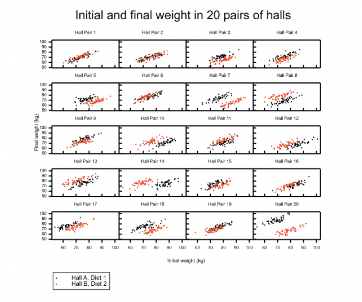
Figure 1 Data for 20 simulated pairs of halls showing final weight plotted against initial weight in the presence of a strong random hall effect.
Figure 1 shows the results of simulating a Lord’s type example using not one pair but twenty pairs of halls. The simulation involves using two bivariate Normal distributions in a hierarchical set-up. In each pair, the hall receiving diet 1 is known as hall A and the hall receiving diet 2 is known as hall B. The true difference between diets is set to be such that, other things being equal, a student receiving diet 2 will be 5kg lighter than if they had received diet 1.
The scatter plots, however, show a bewildering inconsistency given that all 20 pictures represent simulation from identical parameter settings. (In fact, the simulation is produced in one run generating students within one of two halls in twenty pairs.) On many occasions it looks as if diet 2 produces the slimmer students but on many other occasions it is diet 1. This is illustrated in Figure 2, which gives the t-statistic plotted against the estimate for the analysis of each of the twenty hall pairs, conditioning on baseline (as in an ANCOVA). The figure also includes the critical values for ‘significance’ and classifies the results into one of three categories: “in favour of diet 1”, “in favour of diet 2” and “non-significant”. Here a diet is considered favourable if students weigh less under it than they would, other things being equal, on the alternative diet.

Figure 2 t-statistics of the diet effect plotted against the estimate for twenty hall pairs.
Note that, in judging ‘significance’, a Bonferroni correction has been applied to the standard value of 1/40, so for a one sided P-value a result is judged ‘significant’ if P < (1/40)/20 or P > (1/40)/20.
These results show that adjusting for the baseline weight fails to produce any consistent message here, despite producing apparently extremely precise measures. How is this possible? The reason is simple. Allocation to diet is at the level hall not student, yet the analysis attempts to unravel the causal knot at the level of student. This is only possible by making strong assumptions. The assumptions are that a) there is no variation between halls above and beyond the variation between students b) the regression between halls is the same as the regression within. However, I set the simulation parameters to violate both these assumptions.
Note that I am not saying that these assumptions could never be made. They could be, although I personally find assumption a), at least, unlikely to hold in practice. However, I am claiming that Jane’s solution to the problem is not unambiguously wrong. The assumptions should be made explicit so that they are ‘on the table’.
Figure 3 represents the case where I have set the simulation so that there is no random hall effect. Now we can see that there is no problem. Each pair of halls gives the same message: diet 2 leads to a lower weight.

Figure 3 Data for 20 simulated pairs of halls showing final weight plotted against initial weight when there is no hall effect.
Cause fishing with Fisher
One hundred years ago the great statistician RA Fisher arrived at Rothamsted Experimental Research station in Harpenden to start work as their statistician[11]. The whole purpose of Rothamsted was causal: to discover what factors could affect crop growth and yield and to what degree. The whole deep and beautiful field of design and analysis of experiments as developed by Fisher[12], his successors and others working in statistics is devoted to this causal purpose and it is thus rather puzzling to find statistics referred to as a ‘causality-free enterprise’ in The Book of Why (p5). This statement is just wrong.
That statement can be rephrased to make it more reasonable by giving it the qualifier when applied to observational studies, but even here I think this is still something of a calumny. Note that I am not claiming that everything in the causal calculus was anticipated in statistics. Far from it. I consider the development of the calculus and its associated theory by Pearl, his co-workers and those he has inspired to be original, profound and important. However, if it cannot accommodate random effects it is incomplete. In my three previous blogs I showed how application of John Nelder’s experimental calculus produced a solution to Lord’s paradox that, although trivially true in retrospect, is nevertheless evidence of the power of the method.
Finally, I speculate that if the causal calculus can incorporate random effects* it will become even more powerful and useful. Indeed, it is hard to see how the first rung of the ladder of causation, that is to say, association, (Book of Why, p28), can be used without understanding error structures. It has been claimed that all that statisticians taught was that correlation is not causation. However, the truth is far more shocking. What statistics teaches is that frequently correlation is not even correlation. To say that you are adjusting Y for Xi s meaningless unless you say how such an adjustment is to take place. Perhaps the world needs a Book of How.
Postscript
*Since I wrote the first draft of this blog, my attention has been drawn on Twitter to the paper by Kim and Steiner[13], which may address this issue.
Reference
- Wainer, H. and L.M. Brown, Two statistical paradoxes in the interpretation of group differences: Illustrated with medical school admission and licensing data.American Statistician, 2004. 58(2): p. 117-123.
- Lord, F.M., A paradox in the interpretation of group comparisons.Psychological Bulletin, 1967. 66: p. 304-305.
- Senn, S.J., The well-adjusted statistician.Applied Clinical Trials, 2019: p. 2.
- Pearl, J. and D. Mackenzie, The Book of Why. 2018: Basic Books.
- Nelder, J.A., The analysis of randomised experiments with orthogonal block structure I. Block structure and the null analysis of variance.Proceedings of the Royal Society of London. Series A, 1965. 283: p. 147-162.
- Nelder, J.A., The analysis of randomised experiments with orthogonal block structure II. Treatment structure and the general analysis of variance.Proceedings of the Royal Society of London. Series A, 1965. 283: p. 163-178.
- Senn, S.J., Change from baseline and analysis of covariance revisited.Statistics in Medicine, 2006. 25(24): p. 4334–4344.
- Hurlbert, S.H., Pseudoreplication and the design of ecological field experiments.Ecological monographs, 1984. 54(2): p. 187-211.
- Polya, G., How to solve it: A new aspect of mathematical method. 2004: Princeton university press.
- Campbell, M.J. and S.J. Walters, How to Design, Analyse and Report Cluster Randomised Trials in Medicine and Health Related Research. Statistics in Practice, ed. S. Senn. 2014, Chichester: Wiley. 247.
- Box, J.F., R.A. Fisher, The Life of a Scientist. 1978, New York: Wiley.
- Fisher, R.A., The Design of Experiments. 1935, Edinburgh: Oliver and Boyd.
- Kim, Y. and P.M. Steiner, Causal Graphical Views of Fixed Effects and Random Effects Models, in PsyArXiv. 2019. pp. 34. https://psyarxiv.com/cxd2n/
[a]Rothamsted statistics meets Lord’s Paradox https://errorstatistics.com/2018/11/11/stephen-senn-rothamsted-statistics-meets-lords-paradox-guest-post/
[b]On the level. Why block structure matters and its relevance to Lord’s paradox https://errorstatistics.com/2018/11/22/stephen-senn-on-the-level-why-block-structure-matters-and-its-relevance-to-lords-paradox-guest-post/
[c]To infinity and beyond: how big are your data, really? https://errorstatistics.com/2019/03/09/s-senn-to-infinity-and-beyond-how-big-are-your-data-really-guest-post/


")


At this point at least, I find nothing to disagree with here (as usual with your analyses), and in fact am learning from it (as you indicated you did). So my thanks for the posting!
The problem as I currently see it lies with drastic differences in goals, formal models, and languages between you and Pearl. Specifically (and I welcome any correction to my take):
You apply the statistically rich Nelder/random-effects(RE) analysis that provides a Fisherian ANOVA treatment, which is steeped in historical referents and technical facts that I fear will not be understood by most readers to which I (and Pearl) am accustomed.
In contrast, Pearl/Book-of-Why is limited to the simpler more accessible analysis using only expectations under causal models, and so does not address random variability/sampling variation. Thus among other things it does not address certain fixed (“unfaithful”) causal design effects that can arise in designed experiments via blocking or matching. Mansournia and I published a pair of articles about this limitation, not as deep as your analysis but perhaps a bit more accessible (with effort) to those without traditional training in design and analysis of experiments:
Mansournia, M.A., Greenland, S. (2015). The relation of collapsibility and confounding to faithfulness and stability. Epidemiology, 26(4), 466-472.
Greenland, S., Mansournia, M.A. (2015). Limitations of individual causal models, causal graphs, and ignorability assumptions, as illustrated by random confounding and design unfaithfulness. European Journal of Epidemiology, 30, 1101-1110.
Your general point I take it is that the theory in The Book of Why (and indeed in most treatments of modern causality theory I see, including my own) is incomplete for incorporating uncertainties about or variability of material and responses. It is thus (as you say) incomplete for statistical practice, and leaves its use open to missteps in subsequent variance calculations. But my teaching experience agrees with Pearl’s insofar as the target audience is in more dire need of first getting causal basics down, like how to recognize and deal with colliders and their often nonintuitive consequences. In doing so we must allow for lack of familiarity with or understanding of design-of-experiment theory, especially that involving ANOVA calculus or random effects. Thus while I agree The Book of Why seriously overlooks the central importance of causality in that theory, its criticism would be amended by saying that the theory buried causality too deeply within a structure largely impenetrable to the kind of researchers we encounter. Our efforts were intended to bring to the fore crucial aspects of causality for those researchers, aspects that do not depend on that theory and are even obscured by it for those not fluent in it (as some of the controversy surrounding Lord’s paradox illustrates).
The more specific point I think you make is how the randomization in Lord’s Paradox is itself almost noninformative: With only two halls randomized, it is only a randomized choice of the direction of the confounding (formally, just one sign-bit of information) in what is otherwise an observational study for the treatment effect. That being so, any statistical identification of the effect must depend on untestable assumptions beyond the barely informative randomization.
My questions are:
Does any of my description fail to align with your analysis?
Even if it does align broadly, what key details does it miss?
Again, thanks for the post!
Sander, Thanks for this extremely instructive reply. I look forward to reading the paper. I am very happy to reaffirm what I have already stated that statisticians as well as others will benefit from learning from learning about ‘the causal revolution’. However, I am also convinced that what Stuart Hurlbert called pseudoreplication is an important source of error in science https://www.uvm.edu/~ngotelli/Bio%20264/Hurlbert.pdf and that Rothamsted approach is valuable in teaching caution about many of the claims of ‘big data’.
Just a correction to my post: I copied two adjacent articles from 2015 there but I think only the second one (Greenland-Mansournia) is addressing something connected to the current discussion, and even then only in the broad sense of how ordinary causal graphs miss design effects and thus will not suffice for guiding variance computations.
After spending three years writing Fortran code at Exeter University I moved to the Grassland Research Institute in Berkshire, a sister organisation to Rothamsted, in 1977. There I spent five years writing GenStat code and becoming thoroughly immersed in the ideas of Nelder wrt block and treatment structure. At the same time I was working my way through the classic book on experimental design by Cochran and Cox, and in order to make sure that I fully understood the methods I used to invent data that I then analysed with GenStat. GenStat and “Cochran and Cox” are entirely consistent and it is clear that all Nelder was doing was making sure that GenStat was a fit and proper tool for analysing agricultural experiments.These ideas have stayed with me all my life and, before I attempt to analyse data, I always need to understand its structure.
Perhaps it is easier to understand data structure when one sees an agricultural experiment on the ground. Consider, for example two plots of wheat that receive different treatments, with a number of plants being sampled within each plot. The structure of these data is identical to that of Lords Paradox, yet it should be clear that these data are not worthy of analysis. Any number of effects could be confounded with treatment, some obvious, such as one plot being shaded, some less obvious, such as soil fertility, which will vary across the field. So, this is an experiment with two plots, two treatments, and no replication, as is the example in the Lord’s paradox.
To turn my wheat example into a good experiment we need to add extra plots as replicates. A common question is then: how many plots and how many plants per plot? The best experiment will always be one plant per plot (or one student per hall), but this is usually impractical. Reducing the number of plots (halls) and increasing the number of plants (students) per plot (hall) will lead to a poorer experiment. How much poorer will depend upon the ratio of within to between variation.
Red Herring 1: To me this is an experiment with two plots and two treatments and no replication. It is not an observational study. The fact that one diet was used in one hall and a different diet was used in a second hall makes it a designed experiment.
In 1982 I moved to ICI where I was introduced to “Statistical Methods in Research and Production” by O L Davies et. al. (my copy, third edition 1961: first edition 1947). This book was written by ICI employees, including George Box, and is a very good practical guide to use of statistical methods in the chemical industry, where nested designs are very common. Chapter 6 (Analysis of Variance) introduces components of variance on the second page and all the examples are couched in terms of nested error variances, so is entirely consistent with the GENSTAT philosophy.
Thanks for your interesting comments, Peter and the helpful agricultural example. I was at Exeter from 1971-1975, so we must have overlapped.
Comments on “S. Senn: Red herrings and the art of cause
fishing: Lord’s Paradox revisited (Guest post)”
Comment by Judea Pearl
I am elated to have read your latest post on Lord’s Paradox
and to note that not only is your summary concise and accurate,
but it also gives me a pleasant feeling that, this time,
I agree with all your conclusions (modulo a tiny qualification
below)
Here are our four points of agreements:
1.
SS: The fact that these two different analyses lead to different
conclusions constitutes the paradox. We may note that each is
commonly used in analysing randomized clinical trials, say,
and there the expectation of the two approaches would be identical,
although results would vary from case to case[3].
JP: I totally agree
2.
SS: In The Book of Why (BOW) [4], the paradox is addressed and
the conclusion based on causal analysis is that the second
statistician is “unambiguously correct” (p216) and the first wrong.
JP: I stand behind this conclusion as it is expressed in
The Book of Why: ” In this diagram, W_I is a confounder
of D and W_F, not a mediator. Therefore, the second
statistician would be “unambiguously correct”.
3.
SS: In my blog, however, I applied John Nedler’s
experimental calculus [5, 6] …. and came to the conclusion
that the second statistician’s solution is only correct given
an untestable assumption and that even if the assumption were
correct and hence the estimate were appropriate, the estimated
standard error would almost certainly be wrong.
JP: Again, I totally agree with your conclusions. Yet,
contrary to expectations, they
prove to me that The Book of Why succeeded in
separating the relevant from the irrelevant, that is, the
essence from the Red Herrings.
Let me explain. Lord’s paradox is about causal effects
of diet. In your words: “diet has no effect” according to
John and “diet does have an effect” according to Jane.
We know that, inevitably, every analysis of “effects”
must rely on causal, hence “untestable assumptions”. So BOW did a superb
job in bringing to the attention of analysts the fact that the
nature of Lord’s paradox is causal, hence outside the
province of mainstream statistical analysis.
This explains why I agree with your conclusion that “the
second statistician’s solution is only correct given
an untestable assumption”. Had you concluded that
we can decide who is correct without relying on
“an untestable assumption,” you and Nelder would have
been the first mortals to demonstrate the impossible, namely, that
assumption-free correlation does imply causation.
4.
Now let me explain why your last conclusion also attests
to the success of BOW. You conclude: “even if the assumption were
correct, …. the estimated standard error would almost certainly
be wrong.”
JP: The beauty of Lord’s paradox is that it
demonstrates the surprising clash between John and Jane
in purely qualitative terms, with no
appeal to numbers, standard errors, or confidence intervals.
Luckily, the surprising clash persists
in the asymptotic limit where Lord’s ellipses represent
infinite samples, tightly packed into those two elliptical clouds.
Some people consider this asymptotic abstraction
to be a “limitation” of graphical models. I consider
it a blessing and a virtue, enabling us, again,
to separate things that matter (clash over causal effects)
from from those that don’t (sample variability, standard errors,
p-values etc.). More generally, it permits us to separate issues
of estimation, that is, going from samples to distributions, from
those of identification, that is, going from distributions to
cause effect relationships. BOW goes to great length explaining
why this last stage presented an insurmountable hurdle to analysts
lacking the appropriate language of causation.
It remains for me to explain why I had to qualify
your interpretation of “unambiguously correct” with
a direct quote from BOW. BOW declares Jane to be “unambiguously
correct” in the context of the causal assumptions
displayed in the diagram (fig. 6.9.b) where diet is shown NOT
to influence initial weight, and the initial
weight is shown to be the (only) factor that makes
students prefer one diet or another.
Disputing this assumption may lead to another problem
and another resolution but, once we agree with this
assumption our choice of Jane as the correct statistician
in “unambiguously correct”
I hope we can now enjoy the power
of causal analysis to resolve a paradox that generations of statisticians
have found intriguing, if not vexing.
I think it is somewhat dangerous to assume estimation and identification can be cleanly separated, particularly for complex and/or large scale problems. See:
https://arxiv.org/abs/1904.02826
I think it is somewhat dangerous to assume estimation and identification can be cleanly separated, particularly for complex and/or large scale problems. See eg
https://arxiv.org/abs/1904.02826
Looks like the most general paper I’ve seen yet on the statistical limitations of current received causal modeling (“causal inference”) theory.
I noted these small issues in the introduction (I may have missed where they were addressed later):
First, I didn’t see where you defined P before using it.
Then the last sentence says “…we cannot in general trust identifiability results to tell us what can and cannot be estimated, or which causal questions can be answered, without knowing more about the causal functions involved than is usually assumed”:
The “and cannot” seems not quite right – if nonidentification implies nonestimability, nonidentifiability can tell us about a large class of questions that cannot be answered statistically.
Also, the “usually assumed” seems inaccurate insofar as all the applications I’ve seen in social and health sciences use smooth models that fulfill the needed estimability conditions, so in this sense the gap you discuss gets filled in automatically by statisticians applying causal models.
Finally (and this is just a matter of terminology) I missed a note that much of the statistics literature treats identifiability and estimability as synonyms, so it seems causality theory has innocently done the same.
Re MacLaren & Nicholson:
Robins remarked that the problem is discussed in Robins & Ritov (1997). A curse of dimensionality appropriate (CODA) asymptotic theory for semiparametric models. Statist. Med. 16, 285–319.
and in this new paper and its recent cites by Robins et al. at https://arxiv.org/abs/1904.04276
Hi Sander,
Thanks very much for the comments! And sorry for the slow response.
I don’t want to derail this post so I’ll be brief for now. (BTW – I’d love for someone to compare Nelder et al.’s approach to Pearl et al.’s in detail. Surely some clever student can look into this…).
Re
P – I assume you mean the first quote. If so then yep. I’m not sure whether I should define something that appears in a quote by someone else or not, but maybe I should at least mention it.
‘can and cannot’ – agreed. Will fix at some point.
‘Usually assumed’ – this was meant to refer to the theoretical DAG etc literature rather than practice. Humans are great at filling in the gaps (informal to the rescue of the formal!). Will try to make that clearer.
‘Stats literature’ – yeah, frustratingly variable in my experience. And certainly common to just assume identifiability and then consider estimability (without necessarily calling it that). Eg the papers by Bahadur and Savage, Dohono, Tibshirani and Wasserman cited all restrict to identifiable statistical functionals and then consider various impossibility/possibility/sensitivity results for estimation. I think we mentioned at some point that statisticians typically just take identifiability as given. Which relates to one of your comments above – it’s not necessarily that a bunch of this stuff isn’t in the stats literature, it’s that it can be somewhat buried/obscured etc etc.
Re: Robins, thanks for the refs! Will have a proper read soon (I hope…)
Thank you for your interesting comment. The key word in your reply is “asymptotic”. It is used as if this is unambiguous. But there are two possible asymptotic processes we may consider 1) The number of students goes to infinity 2) The number of halls goes to infinity.
Now compare figure 1 and figure 3. If you look at figure 1 you can see that we have a contradiction between the results from pair to pair. Sometimes one diet appears to be better, sometimes another, depending on which pair we look at. This will not be resolved by increasing the number of students. It can only be resolved by increasing the number of halls.
If you look at figure 3, however, you will see that we have already reached the asymptotic paradise that causal calculus assumes we shall be given admittance to if only we follow its rules. There is no need to increase the number of students to get the answer as to which diet is better. Each and every pair gives us the same answer with the number of students we have already studied. We are already, effectively, asymptotic.
So the assumption that Jane makes is that the generating process is such that the situation in figure 3 applies. However, nothing requires this to be so and as the god of this simulation universe I can easily bar her from entering the asymptotic paradise by setting the world to be that represented by figure 1. How can she defeat this ruse of mine? By recognising what the Rothamsted approach teaches. The level at which treatments vary matters.
I suspect that I will not have succeeded in convincing Professor Pearl so let me encourage him to think about one further proposal. Suppose that I can only study a very few students but I say ‘not to worry I can weigh each student dozens of times. I may not have many students but I will end up with a lot of measurements.’ Will this get me my asymptotic answer? If not, why not and what else does it imply?
The whole purpose of statistics was causal (recall Galton and Pearson!), does that means that statistics has developed a language to deal with its purpose? No. It has not. Fisher would have fumbled on Lord’s paradox no less than his modern disciples, who are willing go to all extremes: finite sample, block design, Mendelian randomization, quantum uncertainty, partial diff equations — everything, except learning a language to deal with its purpose – causation. I can only explain this phenomenon by postulating an embarrassment over seeing a century gone by with no language developed to address statistics core purpose – causation. Dennis Lindley was the only statistician I knew who admitted this embarrassment. I am glad to hear (from rkenett ) that Mosteller and Tukey admitted so as well. We are in the 21st Century; can statisticians finally get over this embarrassment and explain to the world why Lord’s paradox is “paradoxical”? Same with Simpron’s paradox and Monty Hall. ???
Senn writes: “The whole purpose of Rothamsted was causal: to discover what factors could affect crop growth and yield and to what degree. ” followed by “The whole deep and beautiful field of design and analysis of experiments as developed by Fisher[12], his successors and others working in statistics is devoted to this causal purpose and it is thus rather puzzling to find statistics referred to as a ‘causality-free enterprise’ in The Book of Why (p5). This statement is just wrong.”
To be fair, this type of statement is not unique to Pearl. Two examples:
Odd Aalen – “Statistics is important because it is conceived as contributing to a causal understanding …Statistics can indicate causality even in the absence of a mechanistic understanding. But the traditional self-conception of statistics is that it can rarely say anything about causality. This is a paradox.” *From a presentation celebrating 50 years to the establishment of a Masters Degree in Statistics in Norway, May 22, 2006.
and
Mosteller and Tukey – “causation, though often our major concern, is usually not settled by statistical arguments” From Data analysis and regression : a second course in statistics, Addison-Wesley, 1977
The underlying issue is that statistics has moved from being a major partner in the discovery process (Fisher…) to being a gate keeper mostly concerned by hygiene and sanitization issues (p< 0.05 or p<0.005). This is where the discussion on causality comes in. Users/customers of statistics expect us to say something related to causality. If we don't, others will….
PS1 The recent ASA initiatives/publications unfortunately reinforce the gate keeper image.
PS2 Our new book on The Real Work of Data Science is about contributing to organisation's bottom line https://www.amazon.com/gp/product/1119570700/ref=dbs_a_def_rwt_bibl_vppi_i0
PS3 Our forthcoming edited book on analytics in the 4th industrial revolution will give a glimpse at what statistics and statisticians can do in this exciting era of sensors, IoT, big data, flexible manufacturing and augmented reality. https://www.amazon.com/gp/product/1119513898/ref=dbs_a_def_rwt_bibl_vppi_i17
My third comment on
S. Senn’s post: Lord’s Paradox revisited.
(posted August 2, 2019 )
———————————————
The upsurge of interest in Lord’s paradox gives me
an opportunity to elaborate on another interesting aspect
of our Diet-weight model, Book Of Why, page 217, Fig. 6.9
Having concluded that Statistician-2 (Jane) is
“unambiguously correct” and that Statistician-1 (John) is
wrong, an astute reader would ask: “And what
about the sure-thing principle? Isn’t the overall
gain just an average of the stratum-specific gains?”.
(where each stratum represents a level of the initial weight
W_I). Previously, in Fig. 6.8, we dismissed this intuition by noting
that W_I was affected by the causal variable (Sex) but, now,
with the arrow pointing from W_I to D we can no longer
use this argument. Indeed, the diagram tells us (using the
back-door criterion) that the causal effect of D on Y
can be obtained by adjusting for the (only) confounder,
W_I, yielding:
P(Y|do(Diet) = SUM_{W_I} P(Y|Diet, W_I) P(W_I)
In other words, the overall gain resulting from administering
a given diet to everyone is none other but the gain observed
in a given diet-weight group, averaged over the weight.
How is it possible then for the latter to be positive
(as seen from the shifted ellipses)
and, simultaneously, for the former to be zero
(as seen by the perfect alignment of the ellipses
along the W_I = W_F line )
Should we conclude that data matching the ellipses
of Fig 6.9(a) can never be generated by the model
of Fig. 6.9(b) , in which W_I is the only confounder?
Impossible! Because we know that the model has no refuting
implications.
The answer is that the sure-thing principle applies
to causal effects, not to statistical associations.
The perfect alignment of the ellipses does not
mean that the effect of Diet on Gain is zero;
it means only that the Gain is statistically
independent of Diet:
P(Gain|Diet=A) = P(Gain|Diet=B)
not that Gain is causally unaffected by Diet.
In other words, the equality above does
not imply the equality
P(Gain|do(Diet=A)) = P(Gain|do(Diet=B))
which statistician-1 (John) wants us to believe.
To conclude, Lord’s paradox started with a clash
between two strong intuitions: (1) To get the effect we
want, we must make “proper
allowances’ for uncontrolled preexisting differences between
groups” (i.e. initial weights) and (2) The overall effect
(of Diet on Gain) is just the average of the stratum-specific
effects. Like the bulk of our mental intuitions, these two are CAUSAL.
Therefore, to reconcile the apparent clash between them we need
a causal language; statistics alone won’t do.
The difficulties that generations of statisticians
have had in resolving this apparent clash stem from
lacking a formal language to express the two intuitions
as well as the conditions under which they are applicable.
Missing were: (1) A calculus of “effects”
and its associated causal sure-thing principle and (2)
a criterion (back door) for deciding when “proper allowances
for preexisting conditions” is warranted. We are now in
possession of these two ingredients, and we should feel
empowered to resolve all paradoxes that surface from the
causation-association confusion that our textbooks have bestowed upon
us.
Professor Pearl uses the word ‘adjusting’ without addressing the issue as to how one needs to adjust. The idea that any adjustment at the level of student is automatically adequate for dealing with treatments that vary at the level of hall is wrong. It requires an untestable assumption. I invite the reader who doubts this to compare figure 1 and figure 3 of the original post. Each figure represents 20 possible realisations of the form of the Wainer and Brown variant of Lord’s Paradox, which will also be found on P216 of The Book of Why.
In figure 3, there is a consistent message. The red points (Hall B , diet 2) lie in a cloud that is regularly below the black ones (Hall A, diet 1). Note, however, that the consistency of the message cannot be seen from looking at one pair only, which is what we have to judge by in the classic two-hall problem. It can only be judged by looking at many pairs, which, given the “design”, we would not have in practice. This is because “hall” is confounded with “diet”. So, without further assumptions we could justifiably come to the conclusion “controlling for weight at the beginning, students in Hall B, diet 2 have lower weight at outcome than those in Hall A diet 1” but we cannot judge that (say) if we switched diet between halls we would find that this association with diet survived and that the association with hall would be broken.
We can see this by looking at figure 1. Here, again we have twenty pairs. Now, however, the apparently convincing picture when one looks at any given panel is inconsistent and this is underlined by figure 2, which shows that on many occasions diet 2 appears to produce lower weights but on other occasions it is diet 1 and on some no clear pattern emerges.
The reason that this happens is that the components of variation and covariation at the level of hall have been set to zero for the case described by figure 3 but not for the situation described by figure 1.
The interesting fact for me, in all this, however, is not so much the solution itself. I consider that that was pretty much complete in the insightful analyses of Holland and Rubin in 1983 (who describe many different variants). I also described a solution using analysis of covariance but also the necessary assumptions in 2006. No, what is interesting is that you can reach this very simply using Nelder’s experimental analytic calculus as incorporated in GenStat.
Unit of inference is an important concept in statistics and the idea that you can somehow escape this when making causal inferences is wrong. It seems that some of the other commentators to this blog, starting with the machinery of DAGs, agree with me.
References
Holland, P.W. and D.B. Rubin, On Lord’s Paradox, in Principles of Modern Psychological Measurement, H. Wainer and S. Messick, Editors. 1983, Lawrence Erlbaum Associates: Hillsdale, NJ.
Lord, F.M., A paradox in the interpretation of group comparisons. Psychological Bulletin, 1967. 66: p. 304-305.
Nelder, J.A., The analysis of randomised experiments with orthogonal block structure I. Block structure and the null analysis of variance. Proceedings of the Royal Society of London. Series A, 1965. 283: p. 147-162.
Nelder, J.A., The analysis of randomised experiments with orthogonal block structure II. Treatment structure and the general analysis of variance. Proceedings of the Royal Society of London. Series A, 1965. 283: p. 163-178.
Pearl, J. and D. Mackenzie, The Book of Why. 2018: Basic Books.
Senn, S.J., Change from baseline and analysis of covariance revisited. Statistics in Medicine, 2006. 25(24): p. 4334–4344.
Wainer, H. and L.M. Brown, Two statistical paradoxes in the interpretation of group differences: Illustrated with medical school admission and licensing data. American Statistician, 2004. 58(2): p. 117-123.
Stephen: I have seem some characterize the present debate as something like “Pearl vs. Nelder”/”DAG vs. Genstat”. I think this framing is a category error in several ways, especially in that your comments emphasize level of analysis as well as effect identification.
Pearl’s only concern is to establish identification in a given causal DAG (cDAG), which can incorporate experimental design features that correspond to deleting arrows (e.g., randomization) but cannot discriminate among design features that lead to the same (or no) deletions and hence the same cDAG. Thus its calculus cannot “see” design features that leave arrows intact but which for example balance effects across paths (and thus it will be blind to their ensuing variance effects).
Nelder is concerned with identification by a given experimental design. He assumes enough regularity to get interval estimability when there is identification – in fact Fisher, Nelder, etc. were almost always operating within ordinary GLMs (linearizable models with exponential-family errors) with identification achieved by having measured without error (or with an estimable error structure) a small yet sufficient set of baseline covariates; the latter identification condition they could at least approximate closely with carefully designed and executed experiments.
As I see it, once one says the question is one of identification, Lord’s Paradox is just a question of which cDAG describes the situation; the do-calculus tells you the form of the target and we can see whether our measurements provide identification, just as Pearl describes. In this respect it is just a variation of the theme in Simpson’s paradox, as Pearl says. The desired interval estimability of that target will ensue with further assumptions. Note that Pearl’s cDAGs for Lord’s Paradox assume there are no other covariates in the problem so the replicate question does not apply to them; with regularity the ensuing interval estimates can be built from the within-treatment variances. Thus it is still is not at all clear to me whether the replicate issue has anything to do with Pearl’s responses or for that matter with the “paradox” Lord raised (especially since his question involved sex effects, which are presumably mediated and moderated but not confounded).
To address the replicate issue, let us focus on the cDAG in this story in which the diet effect on final weight is of interest and thus the central concern is about confounding. In my view the question of replicates vs pseudoreplication is just a variant of whether one has a valid instrument for dealing with uncontrolled potential confounders: The randomized replicate treatment indicator R is such an instrument: R is independent of those potential confounders and has no effect on the outcome other than through the treatment it assigns (monotonicity follows from the perfect compliance assumed implicitly in most of the classic experimental-design literature).
Replicate definition defines the level of effect being estimated; if the replicates are individuals, it is an effect of individual diet assignments that is being estimated; if the replicates are halls, it is an effect of hall diet assignments that is being estimated. The hall-assignment effect may be an average of individual assignment effects, but need not be due to “contextual interactions”, e.g., interactions among hall members having effects on diet compliance and hence the outcome. There are distinct levels for conditions for confounding of these effects; we could for example have no confounding for one and uncontrollable confounding for the other. That fact is often obscured in the so-called ecologic-study literature, so I tried to deconfound it in
Greenland, S. (2001). Ecologic versus individual-level sources of confounding in ecologic estimates of contextual health effects. International Journal of Epidemiology, 30, 1343-1350.
Greenland, S. (2002). A review of multilevel theory for ecologic analyses. Statistics in Medicine, 21, 389-395.
At the individual level considered by Pearl, the replicate issue can now be seen as concerning the question of estimation in the face of a more complex reality than that in those in Pearl’s cDAGs or at the core of Lord’s “paradox” – it goes beyond the paradox to question the very cDAG summarizing the causal data generator, asking “what if the cDAG for the diet-effect target needs an unmeasured U which might be pointing at both diet D and final weight Wf?” We then need to either justify omitting the U->D arrow by randomizing individual diet according to a random individual indicator R, in which case the entire D-Wf association can be attributed to the causal effect of D on Wf; or more weakly find an unconfounded R that will affect Wf only through D (via a monotonic effect of R on D), thus allowing us to attribute an estimable part of the D-Wf association to the causal effect of D on Wf (the first case being the special case in which the effect of R completely displaces the effect of U on D).
After all that, I take it your message is: Hall H is not such an indicator R, given that it may affect Wf via its associated factors. As you emphasize, however, multiple halls can be assigned independently of their characteristics, becoming the replicates, leading to an unconfounded estimate of the effect of diet assignment on units of hall, so that the randomization indicator is now at the hall level. But again, that aggregate-assignment effect should be kept distinct from the effect of assignment of individuals within halls, the estimability of which involves different conditions.
Your (and of course other) reactions to my summary analysis would be of great interest.
In particular: I believe the individual effect is the question Pearl is addressing and that he believes it was the question Lord was addressing – So, can you point to where Lord was instead showing concern with an aggregate-assignment effect?
Thanks, Sander. I regard calculating standard errors (or establishing the degrees of certainty and uncertainty in some other appropriate way) as being a central task of estimation. I fail to see how anyone can combine information from different sources (and that includes prior distribution and data for Bayesians) unless this is done, nor even how they can decide if they have enough information to establish anything useful. So, yes, I am concerned that the correct variances for estimation be established. If this is not of any importance to the Causal Calculus, then Judea Pearl and I, may indeed be talking past each other.
I concede that in some cases correct estimates can be produced even when correct standard errors cannot. Classically, a randomised block design will give. the same estimate as a completely randomised design, although not, in fact, for many Bayesians.
However, this is not the case here. The Book of Why states (p216) “The second statistician compares the final weights under Diet A.to those of Diet B for a group of students starting with weight W0 and concludes that the students on Diet B gain more weight.” What Nelder’s approach shows is that this cannot be done without making special assumptions. This is because diet being varied at the level of dining room* (as per Figure 6.9 on p217) , it is the between-hall regression not the within-hall regression that is important and the latter is not equal to the former except by assumption. Ironically, Figure 6.6 in The Book of Why, in connection with Simpson’s Paradox, shows a case where the within-group regression is not the same as the between group regression.
Anticipating, yet another red herring (not from you but perhaps from others), note that the sure thing principle is not a ‘get out of jail card’ here. In figure 6.6, exercise varies within age groups and the correlation between exercise and cholesterol is negative but overall is positive (because confounded by age). However, in the dining halls example, the putative causal factor varies at the higher level and an attempt is made to study it at the lower level. So, basically, The Book of Why makes the reverse error in figure 6.9 to the one it corrects in figure 6.6.
So it is not just that the Nelder approach shows that we are in danger of getting the standard error wrong. It also shows that we may get the estimate wrong, if we do not take care. So, I stick with my original contention that even if your primary purpose is causal, the Rothamsted approach is useful but since (pace Pearl) Rothamsted’s primary purpose was causal, this is hardly surprising.
So, in summary, my feeling is that some sort of Rothamsted and causal calculus synthesis would be valuable. It may be that your work with Mansournia, for example, may help produce it..
*Lord, used the term ‘dining hall’
Taking a step back, it seems that some of the above arguments come from mixing a perspective of engineering with a perspective of science.
Nozer Singpurwala had some comments related to this in the context of a discussion on the positioning of the field of reliability as science (or not): https://onlinelibrary.wiley.com/doi/abs/10.1002/asmb.2442.
Let me quote him: “The objective of the natural sciences is to devise and refine approximate descriptions or models of physical universe by
1. asking a question;
2. formulating an hypothesis;
3. testing the hypothesis, and then either rejecting it or provisionally accepting it until new evidence forces its modification or its rejection.
Per the Popperian view, science grows by framing hypotheses and subjecting them to increasing severity. Progress is achieved by the fact that each successive hypothesis has to pass the same test as its predecessor, and at least one of those that its predecessor has failed. This view is in contrast with the older view wherein science was about framing laws derived by induction from a multitude of particular and observational facts. To Popper, generalizations comes first and the observations used to test the generalizations come next. From Popper’s viewpoint, this then is the philosophy of science.”
The perspective here is different from what engineering aims at. The Concise Oxford English Dictionary defines it as “the application of science for directly useful purposes…”.
The “statistical limitations of current received causal modeling ” as stated by SG seem to cross the line between these two perspectives.
To paraphrase the above, and to position statistics as a contributor to the discovery process (as mentioned in an earlier blog): “generalizations comes first” .This is where the causality argument comes in and I believe is synergistic to statistical thinking. There is of course the need to discuss estimation and identifiability, but the limitations in this do not diminish the value of the causality argument (at least, to me).
Progress in science, and the application of science for directly useful purposes, do not have to be mutually exclusive. We should however better clarify what is discussed. Severe testing does not seem to be a great concern in engineering.
As a minimal step, we should make sure that terms carry the same meaning in the discussion. To make the point, the paper by Robins & Ritov (1997) A curse of dimensionality appropriate (CODA) asymptotic theory for semiparametric models. (Statist. Med. 16, 285–319) uses an acronym that for many people means Compositional Data Analysis https://www.coda-association.org/en/. The term “adjusting” in SS’s comment is another (weaker) example.
PS Note that the term Severe Testing has been used twice here….
My definition of significance is too hasty. I should have done this in terms of P and 1-P. Basically two one sided tests are carried out. I hope that I have not confused readers too much.
🙂
Dang you Pearl and Senn for making me read and think so much today. They made me go back and re-read “Pseudoreplication and the Design of Ecological Field Experiments”, by Hurlbert, 1984, too
Cheers,
Justin
We have two data sets each consisting of points (x,y) where x is the covariate and y is the dependent variable is taken to be a function f of x, y=f(x). As the data are noisy we include a noise term r giving y=f(x)+r(f,x) where we let r depend on f and x. The question of interest is whether the two data sets can be adequately approximated by the same function f. The reader can reflect at this point as to whether this is, in a sense, really the question of interest. It makes no mention of causality.
The original Lord’s data was simulated by using binormal distributions. The parameters were the same apart from the means mu_x=mu_y=k_b for boys and mu_x=mu_y=k_g ne k_b for hall girls The functions f_b and f_g are of the form
(1) y=f(x)=(rho*sig_y/sig_x)x+mu_x(1-(rho*sig_y/sig_x)).
In Lord’s paradox the first statistician calculates the average change in weight of the boys and of the girls and compares them to give the total effect:
(2) TE=int_supp(x in boys) (f_b(x)-x)h_b(x)dx -int_supp(x in girls) (f_g(x)-x)h_g(x)dx
where supp denotes the supports of the covariate x, h_g the density of the covariate x for boys and h_g the density for girls. As the difference is zero, in the original paradox both expressions are zero, the conclusion is that there is no diet effect. The fact that the integrals are the same does not imply that f_b=f_a even if the supports are equal which in this particular case they are not.
In [] Pearl gives his interpretation of the paradox:
“The research question at hand is whether the weight change process (under a fixed diet condition) is the same for the two sexes. In other words, the question is whether the distinct metabolism of boys has a different effect on their growth pattern than that of girls.”
This suggests that Pearl asks whether the functions =growth patterns are equal but this is not the case. He replaces the total effect by the direct effect defined as
(3) DE=int_supp(x in girls) (f_b(x)-f_g(x))h_g(x)dx
Figure 1 of [1] shows that this is non-zero which implies that the functions are different. However DE=0 does not imply f_b=f_g. There is however a problem with Pearl’s definition which he does not mention. It makes no sense if the supports supp(x in girls) and supp(x in boys) are disjoint. To make sense the integral must be restricted to the intersection of the supports. In the example used for Lord’s paradox this reduces to comparing the heaviest 50% of the girls with the lightest 50% of the boys. The result is still non-zero implying that the functions are not equal.
In contrast the total effect TE makes sense even if the two supports are disjoint. Suppose the heaviest girl has a weight of 65kg and the lightest man of 75kg. In such a case the data provide no information of the effect of the boys diet for weights of less than 75kg and no information of the effect of the girl’s diet for weights greater than 65 kg. Should this give reason to pause? Not at all, the functions are linear so one extrapolates happily in both directions; see Figure 1 of [1]. What happens if it is not linear?
Suppose the y the final weight is given by
(4) y=x+27-2*x^0.6
This function has the property that there is a gain in weight if x 77. Moreover the function looks linear. Suppose all the girls have initial weights of at most 75 and all the boys an initial weight of at least 80. The supports are disjoint. Due to an administrative mixup both get the same diet (4) so there is no diet effect. But both statisticians now conclude that there is an effect: girls gain weight, boys lose weight. The fact that the supports are disjoint doesn’t worry either. If they simply plug everything into their software they may not even notice.
Senn writes about Janes solution:
“However, I am claiming that Janes solution to the problem is not unambiguously wrong. The assumptions should be made explicit so that they are on the table.
So what are the assumptions? That the linear model fits, that I can extrapolate way beyond the support of the data sets. These and others seem not to be on the table. Are they irrelevant?. Does this matter or can we still used the Nelder method even if the data are generated as in (4)?
The Lord’s example is based conceptually and analytically on the linear model. Her is an aside on linear regression. Together with Lutz Dümbgen of the University of Bern I have developed a completely new approach to linear regression. The basic idea is very simple: it compares the covariates with i.i.d. Gaussian covariates. The P-value of a covariate is the probability that the random Gaussian covariate is better, that is gives a smaller sum of squared residuals. It is model free in that the P-values are exact whatever the data. Moreover they agree with those obtained under the standard linear regression model with i.i.d. normal errors. This may be of interest to Mayo. Its main advantage is in the area of covariate choice. It solves the problem of post selection inference PoSI and it can be applied to the case where the number of covariates vastly exceeds the sample size. One example of gene expression data has a sample size of 129 together with 48802 covariates. For such data it outperforms lasso and knockoff in every respect. A paper is available [2] and there is an R package gausscov.
I now move on to more complicated functions In [3] the authors investigate growth
curve for boys and girls. Figure 7 shows the velocity curve averaged over 45 girls. Figure 8 shows the same averaged over 45 boys. Is there a girl-boy effect? It seems that the answer is clear. For example the pubertal peak for boys is large than that for girls. One cannot extract this from considering just integrals. What is the cause? Does it even make sense to talk of cause in this example, at least not for the statistician. The paper uses kernel estimates and parametric fitting, in other words some form of regularization is required. The paper [4] on X-ray diffractograms also involves a nonparametric approach to functions. Again as always some for of regularization is required, in this case minimizing the number of peaks subject to a multiresolution criterion [5]. The paper does not compare different methods of preparing thin films but this can be done. The paper by Omaclaren
https://arxiv.org/abs/1904.02826
cited above considers among other things causality when regularization is required.
I have never felt any need to talk about causality. It is not mentioned in any of the three papers listed below nor in my book. Does this discredit me as a statistician?
[1] Lord’s Paradox Revisited – (Oh Lord! Kumbaya!), Judea Pearl, Journal of Causal Inference, Volume 4, Issue 2, (2016)
[2] A Model-free Approach to Linear Least Squares Regression with Exact Probabilities and Applications to Covariate Selection
Laurie Davies and Lutz Dümbgen
http://arxiv.org/abs/1906.01990
[3] Gasser, Th., Köhler, W., Müller, H.G., Kneip, A., Largo, R., Molinari, L., Prader, A. (1984). Velocity and acceleration of height growth using kernel estimation. Annals of Human Biology 11, 397-411.
[4] Residual-based localization and quantification of peaks in X-ray diffractograms P. L. Davies, U. Gather, M. Meise, D. Mergel, and T. Mildenberger, Ann. Appl. Stat, Volume 2, Number 3 (2008), 861-886.
[5] Local Extremes, Runs, Strings and Multiresolution, P. L. Davies and A. Kovac, Volume 29, Number 1 (2001), 1-65.
Pingback: Causal Analysis in Theory and Practice » Lord’s Paradox: The Power of Causal Thinking
Pingback: Stephen Senn: Being Just about Adjustment (Guest Post) | Error Statistics Philosophy
Pingback: Lord’s Paradox: The Power of Causal Thinking | AIWS.net