

Seeing the world through overly rosy glasses
Taboos about power nearly always stem from misuse of power analysis. Sander Greenland (2012) has a paper called “Nonsignificance Plus High Power Does Not Imply Support for the Null Over the Alternative.” I’m not saying Greenland errs; the error would be made by anyone who interprets power analysis in a manner giving rise to Greenland’s objection. So what’s (ordinary) power analysis?
(I) Listen to Jacob Cohen (1988) introduce Power Analysis
“PROVING THE NULL HYPOTHESIS. Research reports in the literature are frequently flawed by conclusions that state or imply that the null hypothesis is true. For example, following the finding that the difference between two sample means is not statistically significant, instead of properly concluding from this failure to reject the null hypothesis that the data do not warrant the conclusion that the population means differ, the writer concludes, at least implicitly, that there is no difference. The latter conclusion is always strictly invalid, and is functionally invalid as well unless power is high. The high frequency of occurrence of this invalid interpretation can be laid squarely at the doorstep of the general neglect of attention to statistical power in the training of behavioral scientists.
What is really intended by the invalid affirmation of a null hypothesis is not that the population ES is literally zero, but rather that it is negligible, or trivial. This proposition may be validly asserted under certain circumstances. Consider the following: for a given hypothesis test, one defines a numerical value i (or iota) for the ES, where i is so small that it is appropriate in the context to consider it negligible (trivial, inconsequential). Power (1 – b) is then set at a high value, so that b is relatively small. When, additionally, a is specified, n can be found. Now, if the research is performed with this n and it results in nonsignificance, it is proper to conclude that the population ES is no more than i, i.e., that it is negligible; this conclusion can be offered as significant at the b level specified. In much research, “no” effect (difference, correlation) functionally means one that is negligible; “proof” by statistical induction is probabilistic. Thus, in using the same logic as that with which we reject the null hypothesis with risk equal to a, the null hypothesis can be accepted in preference to that which holds that ES = i with risk equal to b. Since i is negligible, the conclusion that the population ES is not as large as i is equivalent to concluding that there is “no” (nontrivial) effect. This comes fairly close and is functionally equivalent to affirming the null hypothesis with a controlled error rate (b), which, as noted above, is what is actually intended when null hypotheses are incorrectly affirmed (J. Cohen 1988, p. 16).
Here Cohen imagines the researcher sets the size of a negligible discrepancy ahead of time–something not always available. Even where a negligible i may be specified, the power to detect that i may be low and not high. Two important points can still be made:
- First, Cohen doesn’t instruct you to infer there’s no discrepancy from H0, merely that it’s “no more than i”.
- Second, even if your test doesn’t have high power to detect negligible i, you can infer the population discrepancy is less than whatever γ your test does have high power to detect (given nonsignificance).
Now to tell what’s true about Greenland’s concern that “Nonsignificance Plus High Power Does Not Imply Support for the Null Over the Alternative.”
(II) The first step is to understand the assertion, giving the most generous interpretation. It deals with nonsignificance, so our ears are perked for a fallacy of nonrejection or nonsignificance. We know that “high power” is an incomplete concept, so he clearly means high power against “the alternative”.
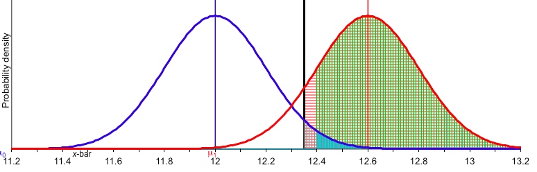
For a simple example of Greenland’s phenomenon, consider an example of the Normal test we’ve discussed a lot on this blog. Let T+: H0: µ ≤ 12 versus H1: µ > 12, σ = 2, n = 100. Test statistic Z is √100(M – 12)/2 where M is the sample mean. With α = .025, the cut-off for declaring .025 significance from M*.025 = 12+ 2(2)/√100 = 12.4 (rounding to 2 rather than 1.96 to use a simple Figure below).
[Note: The thick black vertical line in the Figure, which I haven’t gotten to yet, is going to be the observed mean, M0 = 12.35. It’s a bit lower than the cut-off at 12.4.]
Now a title like Greenland’s is supposed to signal some problem. What is it? The statistical part just boils down to noting that the observed mean M0 (e.g., 12.35) may fail to make it to the cut-off M* (here 12.4), and yet be closer to an alternative against which the test has high power (e.g., 12.6) than it is to the null value, here 12. This happens because the Type 2 error probability is allowed to be greater than the Type 1 error probability (here .025).
Abbreviate the alternative against which the test T+ has .84 power as, µ.84 , as I’ve often done. (See, for example, this post.) That is, the probability Test T+ rejects the null when µ = µ.84 = .84. i.e.,POW(T+, µ.84) = .84. One of our power short-cut rules tells us:
µ.84 = M* + 1σM = 12.4 + .2 = 12.6,
where σM: =σ/√100 = .2.
Note: the Type 2 error probability in relation to alternative µ = 12.6 is.16. This is the area to the left of 12.4 under the red curve above. Pr(M < 12.4; μ = 12.6) = Pr(Z < -1) = .16 = β(12.6).
µ.84 exceeds the null value by 3σM: so any observed mean that exceeds 12 by more than 1.5σM but less than 2σM gives an example of Greenland’s phenomenon. [Note: the previous sentence corrects an earlier wording.] In T+ , values 12.3 < M0 <12 .4 do the job. Pick M0 = 12.35. That value is indicated by the black vertical line in the figure above.
Having established the phenomenon, your next question is: so what?
It would be problematic if power analysis took the insignificant result as evidence for μ = 12 (i.e., 0 discrepancy from the null). I’ve no doubt some try to construe it as such, and that Greenland has been put in the position of needing to correct them. This is the reverse of the “mountains out of molehills” fallacy. It’s making molehills out of mountains. It’s not uncommon when a nonsignificant observed risk increase is taken as evidence that risks are “negligible or nonexistent” or the like. The data are looked at through overly rosy glasses (or bottle). Power analysis enters to avoid taking no evidence of increased risk as evidence of no risk. Its reasoning only licenses μ < µ.84 where .84 was chosen for “high power”. From what we see in Cohen, he does not give a green light to the fallacious use of power analysis.
(III) Now for how the inference from power analysis is akin to significance testing (as Cohen observes). Let μ1−β be the alternative against which test T+ has high power, (1 – β). Power analysis sanctions the inference that would accrue if we switched the null and alternative, yielding the one-sided test in the opposite direction, T-, we might call it. That is, T- tests H0: μ ≥ μ1−β versus H1: μ < μ1−β at the β level. The test rejects H0 (at level β) when M < μ0 – zβσM. Such a significant result would warrant inferring μ < μ1−β at significance level β. Using power analysis doesn’t require making this switcheroo, which might seem complicated. The point is that there’s really no new reasoning involved in power analysis, which is why the members of the Fisherian tribe manage it without even mentioning power.
EXAMPLE. Use μ.84 in test T+ (α = .025, n = 100, σM = .2) to create test T-. Test T+ has .84 power against μ.84 = 12 + 3σM = 12.6 (with our usual rounding). So, test T- is
H0: μ ≥ 12.6 versus H1: μ <12 .6
and a result is statistically significantly smaller than 12.6 at level .16 whenever sample mean M < 12.6 – 1σM = 12.4. To check, note (as when computing the Type 2 error probability of test T+) that
Pr(M < 12.4; μ = 12.6) = Pr(Z < -1) = .16 = β. In test T-, this serves as the Type 1 error probability.
So ordinary power analysis follows the identical logic as significance testing. [i] Here’s a qualitative version of the logic of ordinary power analysis.
Ordinary Power Analysis: If data x are not statistically significantly different from H0, and the power to detect discrepancy γ is high, then x indicates that the actual discrepancy is no greater than γ.[ii]
Or, another way to put this:
If data x are not statistically significantly different from H0, then x indicates that the underlying discrepancy (from H0) is no greater than γ, just to the extent that that the power to detect discrepancy γ is high,
************************************************************************************************
[i] Neyman, we’ve seen, was an early power analyst. See, for example, this post.
[ii] Compare power analytic reasoning with severity reasoning from a negative or insignificant result.
POWER ANALYSIS: If Pr(d > cα; µ’) = high and the result is not significant, then it’s evidence µ < µ’
SEVERITY ANALYSIS: (for an insignificant result): If Pr(d > d0; µ’) = high and the result is not significant, then it’s evidence µ < µ.’
Severity replaces the pre-designated cut-off cα with the observed d0. Thus we obtain the same result remaining in the Fisherian tribe. We still abide by power analysis though, since if Pr(d > d0; µ’) = high then Pr(d > cα; µ’) = high, at least in a sensible test like T+. In other words, power analysis is conservative. It gives a sufficient but not a necessary condition for warranting bound: µ < µ’. But why view a miss as good as a mile? Power is too coarse.
Cohen, J. 1988. Statistical Power Analysis for the Behavioral Sciences. 2nd ed. Hillsdale, NJ: Erlbaum. [Link to quote above: p. 16]
Greenland, S. 2012. ‘Nonsignificance Plus High Power Does Not Imiply Support for the Null Over the Alternative’, Annals of Epidemiology 22, pp. 364-8. Link to paper: Greenland (2012)


")


Greenland’s comments should be viewed in the light of the following remark he makes in the paper,
“The charge of irrelevance can be made against all frequentist statistics (which refer to frequencies in hypothetical repetitions), but can be deflected somewhat by noting that confidence intervals and one-sided p values have straightforward single-sample likelihood and Bayesian posterior interpretations”
for which I have some sympathy.
“The charge of irrelevance can be made against all frequentist statistics (which refer to frequencies in hypothetical repetitions), but can be deflected somewhat by noting that confidence intervals and one-sided p values have straightforward single-sample likelihood and Bayesian posterior interpretations”
I find this strange and interesting, because the only merit I see in Bayesian posteriors and single-sample likelihood is that they can sometimes track with confidence intervals and/or one-sided p-values. Where they do not– and cannot be qualified by error probabilities– I do not see merit. It’s the error probabilities that support any argument for/against merit of the statistical result in the greater context of the scientific questions being addressed.
John:
I can recall Oscar Kempthorne saying something like, if you’re not interested in any classes of possible repetitions of your method, then you don’t have a statistical problem. He visited here many years ago. OK, so I decided not to be lazy and go look up what he said in print. It’s in Godambe and Sprott’s (eds.,) Foundations of Statistical Inference (1971).
“If I am unable to raise his [the scientist’s] interest in any class of repetitions, I shall take the view that he has a unique set of data which cannot be related to other potential sets of data. I shall then say that I am unable to help him, and that…no statistician can hep him.” (p. 490)
But I have heard subjective Bayesians say, in the past at least, that they are interested in the unique and specific data only, and that’s what Kempthorne was reacting to here and in other articles. This would probably sound jarring today, given concerns over replication and reproducibility. The argument for preregistration is based on an appeal to hypothetical repetitions, but recently I’ve started to think that this may be less obvious than it seems. That is why I’ve been working to make such connections explicit (in my new book).
John, if you can only see merit in terms of frequentist error rates then you are more than half blind. There is more than one basis for scientific conclusions, and many circumstances in which error rate considerations are not even a good approach.
Michael: I’m not sure what kind of cases you have in mind. I can agree, as you know, that a crude long-run error justification may be irrelevant, and grant that there are very silly methods with good long-run error rates (flipping a coin and once in a while just “asking Trump” for the measurement of something, while using a highly precise tool the rest of the time, or Kadane’s howler).
But these don’t pass for good tests, and certainly not one’s that satisfy the severity requirement.
Anyway, John was just replying to Grieve’s suggestion that he might have sympathy for the view that hypothetical replications of a method are irrelevant. To that, I gave Kempthorne’s answer last night.
It’s very puzzling when critics complain the p-value isn’t a Bayesian posterior probability of a null hypothesis and also feel the charge can be deflected somewhat by the fact that they can be interpreted that way in confidence intervals and one-sided tests, using vague priors. If the p-value doesn’t give a good measure for posterior belief in the null, it doesn’t become good by invoking a prior that allows it. This isn’t my criticism but many Bayesians raise it.
Good point. It leads me to explain further why I regard Bayesian interpretation of frequentist statistics as useful for applications even when it requires incredible priors.
Briefly, incredible priors warn us to be very careful and elaborate in our frequentist interpretations. In detail:
Inversion fallacies (misinterpretations of P-values as posterior probabilities) have proven fiendishly difficult to eliminate from practice, and are common even in writings by some applied statisticians (the one I see most often treat P as “the probability the results are due to chance”). Nonetheless, posterior interpretations can be used as Bayesian diagnostics, warning the reader that unless backcalculated priors seem reasonable (and that will vary by reader) one should make special effort to stay away from treating P as a posterior probability, and take extra care in providing precise frequentist interpretations.
In regular cases (which are all that I encounter in population-health research) it is easy to backcalculate priors that transform P-values and their corresponding confidence distributions into posterior probabilities. In practice I find that doing so is highly informative for evaluating expert judgment or prior elicitation, a process I see as part of competency in applied statistics (which some label simply as “reasoning under uncertainty”, regardless of formalism or philosophical preference). Even the usual two-sided P-value is a posterior probability; it is just not the posterior probability of a point (since those are all zero in regular cases) – instead in the one-dimensional case it is the limiting posterior probability of two disjoint half intervals (hence it is unsurprising that this interpretation is rarely noted let alone used).
The frequentist interpretation of P-values which I currently find most useful is that P measures distance from the observations to the model space (space of possibilities is being tested). This interpretation (which I see in both Box and Cox at times) supports certain intuitive treatments of P values among experts in applied statistics and avoids common inversion fallacies. Ignoring certain technical issues, one way to operationalize this interpretation is to measure the information in P against the model it tests, for example via the Shannon information (self-information or surprisal) scale S = -log(P), where the usual default base b is 2 in computer science and e in statistical theory.
Under the model constraints, a frequency-valid P-value has a uniform distribution, and -ln(P) has an exponential distribution, so either can be used to measure false-rejection rates.
Nonetheless, the information transform S = -log(P) formalizes how the tested model can only be refuted, never supported by its P-value:
With its information content measured by S, P provides exponentially more information as it approaches zero; the limit P=0 corresponds to logical contradiction between the observations and the model, thus licensing one to declare the model false regardless of one’s error tolerance (alpha level).
In sharp contrast, P=1 corresponds to observations exactly as expected under the model, but the information measure S approaches zero as P approaches 1, and so by the S measure P=1 provides no basis for declaring the model correct.
One way to view this profound information asymmetry between P=0 and P=1 is as follows:
Even if the observations are perfectly consistent with the test model (P=1), there are an infinite number of other models that are also perfectly consistent the observations (this is true even for so-called simple hypotheses since we can always expand the model space, rendering them composite). Under the testing specification, there is insufficient information to discriminate among these models (underdetermination). Put positively, P=1 merely says that there is no information against the test model and thus, absent other information or criteria such as parsimony, this model should be included in future explorations.
The asymmetry between P=0 and P=1 on the Shannon scale interpretations supports common applied intuitions which regard the difference between P of 1 and 0.95 as trivial, yet regard difference between P of 0 and 0.05 as profound. The latter is the difference between outright contradiction of the test model (logical refutation at P=0) and the customary treatment of P=0.05 as borderline evidence against the model (“borderline signficance” corresponding to only -log2(0.05) = 4.32 bits of information against the model).
Contrast these interpretations against typical fallacious interpretations of P=1 such as “the data support the null.” The latter neglects that any support provided by P=1 is smeared out over a practically infinite-dimensional space of possibilities, and that many of these equally supported possibilities are logically inconsistent with the tested model.
+1 for using an information scale. Pure likelihood theory is also quite naturally interpreted as an attempt at an information theoretic approach (valuable for standard practice though I think not quite correct in general)
Thanks omaclaren – I take it we agree that statistics could use more information-theoretic expositions, which can provide valuable ties among frequentist, pure likelihood, and Bayesian perspectives. For example, I have been surprised at some of the claims about ‘information’ in priors voiced by some eminently respectable Bayesian statisticians, even though the claims directly contradict familiar measures such as observed information (which provides a second-order approximation to loglikelihood-based measures) and information-theoretic treatments of Bayesian inference date back at least to the 1950s.
I think that in matters of scientific or contextual interpretation, no formalism is ever quite correct in general (I see failure to recognize this fact as the source of certain practical errors made at times by mathematically rigorous statisticians). The question is then whether the adopted formalism is ‘good enough’ for the application. Deploying several different formalisms can then be seen as a reasonable attempt to hedge against an error in this practical judgment.
So, my question for you (and anyone) is this: What specific limitations of information theory did you have in mind with your parenthetical remark?
> I take it we agree that statistics could use more information-theoretic expositions, which can provide valuable ties among frequentist, pure likelihood, and Bayesian perspectives
Yup, definitely. In fact this is probably the main way that I make sense – and peace with – the various schools of statistics.
> What specific limitations of information theory did you have in mind with your parenthetical remark?
It not so much limitations of information theory per se, but which particular formulations of information theory should be used.
For example, what is the ‘correct’ measure of information? Log probability is reasonable within the context of a well-chosen model but you have to be careful in general to have pre-chosen a good ‘signal vs noise’ decomposition i.e. distinction between regularity and randomness.
Depending what choices are made in measuring information you might end up with a string of numbers with many obvious regularities being considered to contain the same information as a seemingly highly random string, or even a having ‘purely random’ string being considered as containing more ‘information’ than a highly regular string of numbers.
Sander: Let’s see if we can clear up the ONE main question before going on to others: Do you agree that the correct interpretation of power analysis as given by Cohen avoids the counterintuitive case you mention, in the sense that one is not licensed to make even the comparative inference? I don’t doubt some have misused power analysis.
Sander: Although I’ve heard you say the kind of thing you said (in response to E. Berk) before, I continue to view it as zany. It’s to say, we deny the relevance of the error probability meaning that is intended by the p-value, but what makes this irrelevance not really so terrible is that in one-sided and various other cases the p-value does equal a posterior probability in the null, and thus if you find the p-value doesn’t feel attuned to your degree of belief in the null, then you get the benefit of realizing you shouldn’t have interpreted the p-value as a posterior. Does this make sense? So having gone through that little game can you then go back to properly interpreting it as an error probability? The cases where you get a match between p-values and a posterior, the prior is improper and not considered to be representing beliefs. So it’s like saying, the p-value can be of value because since it equals a posterior that would result under a prior that doesn’t represent beliefs, it warns you not to interpret the p-value as a posterior. And if it did seem to reflect one’s degree of belief, then I spoze it’s ok to view it as a posterior? Zany at best.
Mayo – it is clear that the underlying theme of Sander’s comment is information theoretic. If you attempted to understand his comment through these lenses it might make more sense to you. It certainly does to me, despite some misgivings I expressed above.
Most scientists, engineers and mathematicians I’ve encountered are generally more sympathetic to information theory presentations than frequentist or bayesian approaches. The connections between likelihood approaches and information theory has similar appeal I’ve found (and I mean look at how much Fisher refers to information!) among the same group. Hence this is currently my favoured approach (plus simulation) for intro courses. Used it for software engineers recently and I think went well.
Again, though, I think there are some limitations to this approach that Laurie has convinced me of.
Om: Sorry, perhaps I should have made it clearer than I did that I was only referring to the specific response to E. Berk. I have no problem seeing p-values as distance measures (between the observed and the hypothetical distribution of results, assuming the data are generated by a system approximating the null). To me that shows the relevance of distributions of possible outcomes.
I think it goes beyond this though.
E.g. his follow-up to me:
“I take it we agree that statistics could use more information-theoretic expositions, which can provide valuable ties among frequentist, pure likelihood, and Bayesian perspectives.”
Om: I think that’s general enough to assent to. I think the Grieve comment directed us a little bit away from the point of the post. But I admit it has been on draft for awhile, and I’ve already made the point in communications with Greenland some months ago. But I’d still find it useful if he granted that his concern about the use of power analysis disappears if we use power analysis correctly.
That doesn’t mean I wouldn’t want to do even better (by considering the value of the nonsignificant result). I’ll explain this in a later post.
omaclaren
If you are not aware, Richard McElreath also uses information theory in his intro book and course videos http://xcelab.net/rm/statistical-rethinking/
Mayo: Thanks – I’m afraid however from what you wrote I can’t see that you understood what I wrote or are addressing the points I was making, nor do I see clear logical content in calling something “zany.”
So let me try again to explain my points:
First, let me emphasize once again that I in no way deny the relevance of any logically sound interpretation of a P-value or the like, including its correct usage in terms of error probabilities e.g., as in Lehmann’s textbook, where it equals (but is not logically identical to) the smallest alpha level at which we’d reject the test model were we in an NP decision problem. And I honestly cannot see where you got from anything I’ve written that I “deny the relevance of the error probability meaning that is intended by the p-value.” I acknowledge that such denials exist and so must be accommodated, but this quote from you does not represent my own views.
That said, I also have no objection to interpreting P-values as limiting posterior probabilities – as long as the prior sequence which yields that interpretation is clear to the reader (so that the reader can use or ignore that interpretation accordingly).
Second, the point of my initial post here (responding to Berk) was to describe the interesting consequences of adopting the surprisal/Shannon/self-information scaling S = -ln(P) to measure the information encoded in P against the tested model. As an addendum, I should emphasize that (as in Greenland, Senn, Rothman, Carlin, Poole, Goodman & Altman, American Statistician 2016) that model includes all the constraints used to derive the P-value, not only some privileged null hypothesis. I was not rejecting other interpretations such as yours, but instead was pointing out one (of the many legitimate interpretations) which seems unduly neglected in typical debates I see.
This information interpretation of P side-steps the posterior interpretation and applies whether or not the latter is reasonable.
It also side-steps the dichotomization forced on us by the decision-theoretic framework of basic NP theory (which as even Fisher conceded might be useful for automated acceptance sampling, although apparently Deming expressed doubts about that). It is thus is acceptable under the inference-continuity principle that both omaclaren and Lew endorse along with me.
It is far from new and in no way in conflict with traditional Fisherian interpretations, it merely provides a scale (in bits or nats or Hartleys) on which to formalize Fisher’s intuitive use of P to measure “evidence against the null” – In fact Fisher used it to combine information across independent studies, albeit without the later Shannon interpretation. This scale makes precise the senses in which P=0.05 is borderline (only ~4 bits) and the much discussed 5 sigma in physics (~20 bits under normality) or 6 sigma in QC (~30 bits) are clear evidence in the observations against the tested model, apart from any prior. And to the best I can perceive it appears to track the intuitive uses made of P values among paradigmatic practitioners (like Box, Cox, and Fisher at his best), who strive to avoid inversion fallacies.
As omaclaren indicated, there are a huge number of technical issues that can arise with information measurement (especially in continuous models – some of which lead back into Bayesian interpretations, as in Jaynes). Nonetheless, just as with other interpretations, I think those technical problems are far afield from our concerns here, which is how to provide an intuitively satisfying yet logically sound interpretation of P-values without bringing in prior or posterior probabilities.
Let me conclude by observing that in these foundational debates there seems to be another pair of fallacies – or rather, cognitive biases – which seem even less successfully avoided than inversion fallacies:
The first is the exclusivity fallacy: That alternative interpretations are mutually exclusive (and so if one adopts one interpretation one is enjoined from using any other). In reality, logically sound interpretations tend to be mutually consistent, and claims they of conflict are usually traceable to failure to map correctly between the interpretations (a failure which often stems from failure to recognize all the free parameters in the formalizations).
The second (which pairs with the first) is the exhaustiveness fallacy: That the interpretations under debate exhaust all the possible interpretations. This fallacy is usually unrecognized until its circumvention; the latter is popularly labeled “thinking outside the box” (of currently debated possibilities). The fallacy should be easily dispelled by exhibiting a possibility not in the “current discussion” box, which is what I was trying to do for non-Bayesian interpretations of P-values; I am grateful to omaclaren for recognizing this attempt as such.
Sander: Just to get to your first main point since I promised I’d go to sleep early: I do not say that you “deny the relevance of the error probability meaning that is intended by the p-value.” It was Andy Grieve who started off on that in commenting on something you say in your paper:
“The charge of irrelevance can be made against all frequentist statistics (which refer to frequencies in hypothetical repetitions), but can be deflected somewhat by noting that confidence intervals and one-sided p values have straightforward single-sample likelihood and Bayesian posterior interpretations”
My reply was that I didn’t think you regarded sampling distributions and such as irrelevant. So, you’d have to look at the first comment. I will carefully read the rest of your latest tomorrow.
Sander:
I don’t think I disagree with the rest of your comment. The point of the post was to address a gripe of yours, that you’d mention more than once, and the main thing is to show that whoever you have in mind who is guilty of making molehills out of mountains, they would be wrong to suppose ordinary power analysis permits it. (I can’t recall if it comes up again in your most recent group paper.)
“It also side-steps the dichotomization forced on us by the decision-theoretic framework of basic NP theory (which as even Fisher conceded might be useful for automated acceptance sampling, although apparently Deming expressed doubts about that).”
I guess I don’t see any dichotomization “forced on us” by N-P theory. Besides, N-P theory didn’t do just one thing. Neyman, at the same time as developing tests in order to improve and justify Fisher’s tests–sidestepping the problems we see in NHST today–developed confidence intervals. By considering the potential parameter values that are not statistically significantly different from a given outcome, at a given level, you get a corresponding confidence interval. And by varying the different significance levels, one gets a series of confidence intervals. Both N and N-P explicitly rejected the idea of using a single tool for inquiry, and looking at their applications makes this clear.
It seems to me that likelihood ratios, Bayes factors, model selection techniques are binary: which is better M1 or M2? Maybe neither.
Finally, the decision-theoretical development with Wald, and developments by Lehmann were later, although people speak of N-P-Wald.
By the time Fisher was yelling about “acceptance sampling” the radical break (1935) had occurred and the methods he welcomed in 1933 and 34 were, if they were Neyman’s, bad, bad, bad. What’s the Deming reference by the way? (Ironically, E. Pearson (1955), who told Fisher that the behavioristic interpretation of tests was purely Neyman’s, and he wanted no part of it*, is the one who worked in quality control many years before. He wrote 2 books on it, one burned up in a fire, only a small one survives**.)
* http://www.phil.vt.edu/dmayo/personal_website/Pearson%201955.pdf
In a snippet of from Pearson in this post: https://errorstatistics.com/2015/04/24/statistical-concepts-in-their-relation-to-reality-by-e-s-pearson/ “In the first place it seems unfortunate that much of Fisher’s criticism of Neyman and Pearson’s approach to the testing of statistical hypotheses should be built upon a “penetrating observation” ascribed to Professor G.A. Barnard, the assumption involved in which happens to be historically incorrect. There was no question of a difference in point of view having “originated” when Neyman “reinterpreted” Fisher’s early work on tests of significance “in terms of that technological and commercial apparatus which is known as an acceptance procedure”. There was no sudden descent upon British soil of Russian ideas regarding the function of science in relation to technology and to five-year plans. It was really much simpler–or worse. The original heresy, as we shall see, was a Pearson one!” (Pearson 1955)
The “heresy” Pearson has in mind was introducing an alternative, not interpreting the tests behavioristically, which wasn’t part of the original formulation of tests.
**See p. 110 of my exchange with Cox :http://www.rmm-journal.de/downloads/Article_Cox_Mayo.pdf
Concerning “the probability ‘the results’ are due to chance”, I wanted to cite my post on this, for anyone interested:
Andrew: Much of today’s handwringing about statistical inference reflects a concern with gambits that make it too easy for methods to erroneously output some impressive seeming finding or other in hypothetical repetitions. The effects of cherry-picking, data-dependent subgroups, multiple testing, trying and trying again, etc. are reflected in what would occur in replications (as captured in the relevant sampling distribution). If one deems such concerns irrelevant, it’s hard to see how one either assesses or controls a method’s capacity to have revealed flaws in the case at hand. So I hope you don’t have too much sympathy with ignoring hypothetical repetitions. As for Greenland, he has often pointed up passages in his writings that underscore the crucial importance of controlling error probabilities.
Here’s one he cites with Robins:
Click to access greenland-robins-1991-eb-multiple-comp-epidemiol.pdf
This post has been on draft for awhile, so I’d need to reread this particular paper of his to see if it’s anomalous in that regard. I hope others will have a look at it over the weekend.
All that said, it’s not the most direct issue of the post, except in the sense that power analysis gives another use of hypothetical repetitions, even when there’s no issue about data-dependent selection effects.
I cannot resist pointing out that the example used demonstrates that whole problem of interpretation of results that are non-significant in a hypothesis test becomes trivially easy, and notably free of confusing elements when the results are viewed as a likelihood function. The observed value of 12.35 is the possible value of mu best supported by the evidence in the data, but that support is only marginally more than the support for other interesting values such as 12 and 12.6. In that way the likelihood function make it clear that the evidence is insufficient to support strong distinctions between those values and so additional evidence should be gathered or conclusions should be restricted to values of the parameter that differ more widely. No viewer of that function — naive or sophisticated — would be misled into thinking that the data provide strong enough reason by itself to discard any two of those parameter values and retain another.
In that previous paragraph, the evidence is insufficient only in the context that some decision or belief is to be formed on the basis of those data alone. If there is other information that is relevant, or if there is a reason to prefer, for example, a false inference in favour of 12 over a false inference in favour of 12.6 then that information or loss function can be combined with the data-derived evidence about the parameter value and a reasoned argument towards a conclusion can be put.
Michael: Yes, Greenland did frame the problem as a comparative likelihoodist (in his title), but there’s no disagreement about the fact that the data are closer to this particular alternative (that I chose) than to the null*. But Royall, Sober and other likelihoodists (you can tell us if you disagree) say they are unable to handle composite tests, like this one. Royall doesn’t conclude that his test comes up short but rather claims that any genuine test should be restricted to comparing a fixed x to H versus some point alternative H’ (Statistical Evidence,Royall 1997, pp. 19-20).
The reason he gives is that there are parameter values within composite alternative H1 that are even less likely on the data than the null. In his view,then, to assert there’s evidence of some positive discrepancy from 12, is to assert every parameter point within H1 is more likely than every point in Ho! That seems an idiosyncratic meaning to attach to “infer evidence of θ > 12”, doesn’t it?
Nor does it explain what the problem is for the significance tester who does test composite alternatives, because we can also use power (or severity) analysis to avoid declaring there’s evidence of, say, 13, based on a statistically significant result of 12.4. The probability of a larger difference than 12.4 is ~1, were we in a world where θ =13. So the supposed problem is gotten out of (even though it’s not the only way). The other thing is that even though theta = x gets maximal likelihood, to infer a discrepancy that large would be to err ~50% of the time. So we really are doing different things in our inferences.
*This happens here because the type 1 error probability (.025) is smaller than the type 2 error probability (.16).
“The whole problem of interpretation of results that are non-significant in a hypothesis test becomes trivially easy, and notably free of confusing elements when the results are viewed as a likelihood function.” That remains true if we change likelihood to “continuous,” as in:
The whole problem of interpretation of results that are non-significant in a hypothesis test becomes trivially easy, and notably free of confusing elements when the results are viewed as a continuous function over the model space. It applies to P-value functions/confidence distributions as well as to likelihood functions. The only reason P-values seem so troublesome in this regard is the entrenched tradition of dichotomizing them into reject/don’t reject followed by the careless transformation of “don’t reject” into “accept” outside of a strict acceptance-sampling framework. If likelihoods had instead become the convention and were dichotomized in this way, they would have been as misleading and confusing in practice.
Note that in saying this I am not being critical of direct likelihood interpretations. I am only rejecting the notion that such interpretations intrinsically address the fallacies that plague P values – they don’t, and if dichotomized for a decision rule (as in the NP lemma) likelihoods could be misused as badly as P-values (that this hasn’t happened is just an historical idiosyncrasy). Same for posterior probabilities.
> The whole problem of interpretation of results that are non-significant in a hypothesis test becomes trivially easy, and notably free of confusing elements when the results are viewed as a continuous function over the model space
Exactly! ‘Continuity of analysis’ is the most important principle here.
(That is to say, following for example Hadamard – https://en.wikipedia.org/wiki/Well-posed_problem – we might say that we want the results of our analysis to have a continuous dependence on the elements of our setup. Including variations in the given data, model structure etc.
In general this will only ever be ‘local’ in the sense that it will be impossible to rule out all possible directions of instability. Funnily enough this is all part of the ‘numerical continuation’ approach to bifurcation theory in dynamical systems – https://en.wikipedia.org/wiki/Numerical_continuation)
omaclaren:
‘Continuity of analysis’ – agree but I think it needs to be highlighted that the continuity is for the _space of possibilities_ not actualities.
Possibilities are various entertained representations of reality or models where as actualities are our (more) brute force experiences of reality or likely constraints or reality (i.e. observations being being of limited accuracy and hence discrete and constraints making say underlying rates of infections limited to rational numbers.)
So likelihoods are properly defined as probabilities of observations (hence discrete) and parameter spaces of unknowns in reality are actually discrete. But continuous models are far more convenient and productive models of the first and required by principle for the second as _we_ can’t rule out any value before hand and so must allow them all for possibilities.
(Now this was long but it relates to Mike Evans view on insisting on continuous models that remain good approximations for finite models.)
Keith O’Rourke
Hi Keith,
Thanks for your comment. I agree that the continuity is respect to possibilities and that our direct observations may typically be discrete. On the broader philosophical view of eg Evans, you and Jaynes prioritising discrete/finite as fundamental I can’t really agree (not that it matters here!). There are numerous theoretical physicists who would say the discrete arises from the continuous not vice versa. I find this general view of continuity as primary aesthetically pleasing. Incidentally I believe Peirce would likely agree?
But of course we don’t really know either way. And interesting survey of some issues is JL Bell’s ‘The Continuous and the Infinitesimal in Mathematics and Philosophy.’
From memory he has some Peirce references.
> Peirce would likely agree?
Its always a insurmountable challenge to get Peirce right – see below.
My comment was motivated by Peirce’s work (via Paul Forster U of Ottawa) and I carefully said “experiences of reality” rather than reality itself but my constraints or [of] reality was sloppy (along with the typo of or for of).
For keeping to rational numbers for underlying rates (which may be continuous in reality) I should have said unless our powers of discrimination continue to increase without bound our experiences of reality will no longer provide any sense of being wrong somewhere somehow – if investigators hit upon a rational number close enough. But then 100 billion years from now is not a big concern for me 😉
But agree reality may be continuous and I believe pierce though so.
I have yet to read Peirce’s Clarifications of Continuity Jérôme Havenel http://www.jstor.org/stable/40321237?seq=1#page_scan_tab_contents that provides an argument that Peirce changed his view in 1908 nor may have JL Bell.
Keith O’Rourke
(If you do read it perhaps comment here or email me)
Sander, you make a very good point here. Yes, it is the dichotomisation that is at the root of the problems, and P-value functions are a far better option, particularly as they can be interpreted as approximate likelihood functions in many cases.
(I will point out that it was my intention that “likelihood function” implies continuous function where the parameters are reals.)
Yes, and even I can see that. Your simulations show the relationship between likelihood and p-values, and support the intuition that dichotomization will often distort understanding what the data can tell you. My support for p-values never meant I see no value in the likelihood curve and severity curve when interesting results.
Mayo wrote this in a summary response to Sander” “It seems to me that likelihood ratios, Bayes factors, model selection techniques are binary: which is better M1 or M2? Maybe neither.”
Give the discussion of continuity above, and my repeated entreaties over several years that the whole likelihood function be inspected, that statement seems perverse. Mayo might choose to focus all of her attention on a single pair of likelihoods, but Fisher, Edwards, Royall and Pawitan all focus on entire likelihood functions and, at least to my reading, make it perfectly clear that the likelihood function should be interpreted as a continuous function. No-one should make the mistake of assuming that a likelihood analysis yields a binary outcome.
Indeed, the binary interpretation of likelihood ratios seems to be more implied by Pearson’s introduction mention by Mayo above – which is better H0 or H1? Use a likelihood ratio test?
Like I’ve said, I have some concerns about the likelihood approach but they are certainly not based on likelihoodists promoting a binary view. Just read Edwards and Pawitan, like you say. Continuous functions of parameters everywhere. In fact the whole ‘no composite hypotheses’ component of the likelihood approach is due to this – you can’t ask ‘what is the value of a function of one variable at point 1 and at point 2 simultaneously’ as it doesn’t make sense.
This is in response to Michael, but I don’t know if it’s in order:
Royall will contrast his view with significance tests by means of a test of H0: θ ≤ 0.2 vs H1: θ > 0.2 , where θ is the “success probability associated with a new treatment” (in a Bernoulli model). Royall considers a result that reaches statistical significance at level ~.003. While the significance tester takes this as indicating evidence for H1, “the law of likelihood does not allow the characterization of these observations as strong evidence for H1 over H0 (Royall 1997, p. 20). [He uses H1 and H2.] Why? The problem is that even though the likelihood of θ = 0.2 is small, there are values within composite alternative H1 that are even less likely on the data, for instance θ = 0.9.
This is supposed to show a problem with significance tests, because sig tests are not comparative (even though they have an alternative, the composite one). This would be to say that rejecting H0: θ ≤ 0.2 and inferring H1: θ > 0.2 is to assert every parameter point within H1 is more likely (or better supported) than every point in H0. That seems an idiosyncratic meaning to attach to “infer evidence of θ > 0.2”. It doesn’t explain what the problem is for the significance tester who just takes it to mean what it says:
To reject H0: θ ≤ 0.2 is to infer some positive discrepancy from .2.
And a proper use of tests (admittedly Fisher didn’t require it) would indicate that there’s terrible evidence for θ = 0.9; you’d expect observed proportions greater than observed with probability ~1 were the data to have come from θ that large.(I’m not giving the specifics of the outcome, you can check the page.)
He does say that he can give the likelihood ratios of “the totality of possible values of θ” (p. 20) so if he were to allow composite inferences, with the qualifications of which alternatives are better supported than the null, it seems we’re not so different after all, except for two things: (1) Hypotheses to which he’ll give maximum comparative support are ones for which we’d say there’s poor evidence and (2) He will not differentiate cases where the alternative is a data-dependent selected hypothesis. To take his example, success associated with a new treatment can be measured in scads of different ways. That’s why it’s usually required to preregister what features are going to be measured in determining success. Otherwise there’s a high probability of finding success on some feature or other, even if it’s due to chance variability. Royall could not be more dismissive of such error statistical reasoning. If you don’t like the data-dependent alternative, it must be because you give it a low degree of belief. But it’s not belief–it’s the method that bothers us.
With 2 prespecified hypotheses there’s error control (and to some extent with finitely many prespecified hypotheses—yet the error control goes down the more there are), but if it’s open-ended there is not. That’s why binary choices are the typical form–but there’s no onus on predesignation. Now Lew will say that I’m entering the land of “action”, but I’m interested in inference. Even if we suppose there’s no issue of selection effects or stopping rules (which is to sidestep a central problem of statistical inference), we at most have a report of data and are still in need of an account of inference. By Royall’s own admission, his other categories do not count as inferences about what’s warranted by evidence. Perhaps this is the place that Lew can improve on existing Likelihoodlums.
Sorry this got long, and no time to proof it.
> Perhaps this is the place that Lew can improve on existing Likelihoodlums
I would suggest instead that the easiest way to improve on *your account* of existing ‘Likelihoodlums’ would be to read Edwards and Pawitan in detail, work through their examples and give a detailed comparison of your severity analysis on these specific examples.
Also, when you say
> He does say that he can give the likelihood ratios of “the totality of possible values of θ” (p. 20) so if he were to allow composite inferences, with the qualifications of which alternatives are better supported than the null, it seems we’re not so different after all, except for two things…
This suggests that you are surprised that a Likelihoodist would present a likelihood function – i.e. plot the (normalised) likelihood as a function of the parameter for all possible values of theta. This is in fact the standard likelihood approach, especially if the goal is not a comparison with frequentist tests but simply to work within the paradigm.
Om: I’ve given my critique: no or limited error control. That’s why I say it fails as an account of inference in an essential way. It’s fine and informative to look at likelihoods and various other types of data analysis, but for ampliative inference–inference that goes beyond the data– we need an account that enables evaluating and controlling the probabilities of erroneous interpretations of data. The LL doesn’t do this, and for some odd reason, its adherents disparage that goal.
There’s a reason one-time likelihoodists like Hacking, Birnbaum, Barnard move away from a likelihoodist account. Here’s Birnbaum in the same issue of BJPS in which Hacking reviewed Edwards, declaring he’d given it up. I’ve added the Hacking link.
Click to access hacking_review-likelihood.pdf
I realize we’ve gotten way off topic.
Again, I would simply suggest that anyone interested in a proper understanding of the Likelihoodist approach read the actual books by Edwards and by Pawitan in particular, work the examples, compare to other approaches yourself.
As I’ve said, I have my issue with pure Likelihoodist approaches, but I do find them quite appealing in many respects. And certainly suggestive of fruitful directions, even if you end up with something else.
As Hacking’s review concludes:
“I hope Edwards’s book will encourage others to enter the labyrinth and see where it goes”
Also worth pointing out that Edwards believes that Birnbaum ending up reinventing Fisher’s Fiducial inference after he abandoned likelihood. Senn has previously commented on the similarities of severity to Fiducial inference, and I’ve tried to make the same point before. The problem is, Fiducial inference and Confidence inference (and effectively Bayes and Likelihood) are all basically essentially identical for the simple examples considered by Mayo. In order to better distinguish the approaches we need at least one non-trivial example of severity analysis.
Om: I don’t think people have trouble seeing they are all wildly different in interpretation, even when we get so-called”agreement on numbers”. We just saw this with Royall’s little example. But we usually don’t get agreement. Don’t you remember the zillion posts on p-values exaggerate? There was both disagreement on numbers and interpretation. Just about every debate on foundations revolves around simple examples. The rationale given by many, and I agree with them, is that if you’re trying to focus on the logic, you don’t want extraneous complexities entering. All these approaches disagree on testing assumptions, though I’m not sure if likelihoodists test model assumptions. Give me an example of the sort you have in mind.
How about a problem with a single nuisance parameter. RE: Royall etc, I have seen any evidence you understand the Likelihoodist approach.
*meant haven’t, obviously
Om: You’re confusing much more general accounts that focus on likelihood and the much narrower accounts following the Law of Likelihood as with Royall.
Some discussion of nuisance parameters (Starting Section 9):
Click to access ch%207%20cox%20&%20mayo.pdf
None of this discussion pertains to the topic of the post.
See Sander’s comments on exclusivity and exhaustivity above. I also maintain that you are either misrepresenting or misunderstanding the Likelihoodist position (for one example). Since you are fond of referring to reviews I’d suggest people read Edwards’ review of Royall’s book.
I don’t generally have any big issues with your approach on the simple examples I’ve seen – though still I fail to see how you would intend it to apply to anything beyond a normal distribution with unknown mean. My biggest problem is how you present other approaches such as Bayesian and Likelihoodist etc. If people were to rely on your accounts rather than read the best presentations by the main advocates they would get a very misleading view (of course, same applies to eg many accounts of Frequentist inference by Bayesians).
I’m interested in an honest appraisal of the merits and troubles of various approaches by those with a genuine desire to understand. That these discussions end up about debate tactics, rhetoric, picking a team etc is very disheartening.
People like Sanders are rightly commended for giving each approach proper consideration, being open to other points of view and testing out methods by putting them to ‘severe test’ – seeing how they stand up against non-trivial problems.