

.
Suppose you are reading about a statistically significant result x (just at level α) from a one-sided test T+ of the mean of a Normal distribution with n iid samples, and (for simplicity) known σ: H0: µ ≤ 0 against H1: µ > 0.
I have heard some people say [0]:
A. If the test’s power to detect alternative µ’ is very low, then the statistically significant x is poor evidence of a discrepancy (from the null) corresponding to µ’. (i.e., there’s poor evidence that µ > µ’ ).◊See point on language in notes.
They will generally also hold that if POW(µ’) is reasonably high (at least .5), then the inference to µ > µ’ is warranted, or at least not problematic.
I have heard other people say:
B. If the test’s power to detect alternative µ’ is very low, then the statistically significant x is good evidence of a discrepancy (from the null) corresponding to µ’ (i.e., there’s good evidence that µ > µ’).
They will generally also hold that if POW(µ’) is reasonably high (at least .5), then the inference to µ > µ’ is unwarranted.
Which is correct, from the perspective of the (error statistical) philosophy, within which power and associated tests are defined?
Allow the test assumptions are adequately met. I have often said on this blog, and I repeat, the most misunderstood and abused (or unused) concept from frequentist statistics is that of a test’s power to reject the null hypothesis under the assumption alternative µ’ is true: POW(µ’). I deliberately write it in this correct manner because it is faulty to speak of the power of a test without specifying against what alternative it’s to be computed. It will also get you into trouble if you define power as in the first premise in a recent post:
the probability of correctly rejecting the null
–which is both ambiguous and fails to specify the all important conjectured alternative. [For handholding slides on power, please see this post.] That you compute power for several alternatives is not the slightest bit problematic; it’s precisely what you want to do in order to assess the test’s capability to detect discrepancies. If you knew the true parameter value, why would you be running an inquiry to make statistical inferences about it?
It must be kept in mind that inferences are going to be in the form of µ > µ’ =µ0 + δ, or µ < µ’ =µ0 + δ or the like. They are not to point values! (Not even to the point µ =M0.) Most simply, you may consider that the inference is in terms of the one-sided lower confidence bound (for various confidence levels)–the dual for test T+.
DEFINITION: POW(T+,µ’) = POW(Test T+ rejects H0;µ’) = Pr(M > M*; µ’), where M is the sample mean and M* is the cut-off for rejection. (Since it’s continuous it doesn’t matter if we write > or ≥). I’ll leave off the T+ and write POW(µ’).
In terms of P-values: POW(µ’) = Pr(P < p*; µ’) where P < p* corresponds to rejecting the null hypothesis at the given level.
Let σ = 10, n = 100, so (σ/ √n) = 1. (Nice and simple!) Test T+ rejects H0 at the .025 level if M > 1.96(1). For simplicity, let the cut-off, M*, be 2.
Test T+ rejects H0 at ~ .025 level if M > 2.
CASE 1: We need a µ’ such that POW(µ’) = low. The power against alternatives between the null and the cut-off M* will range from α to .5. Consider the power against the null:
1. POW(µ = 0) = α = .025.
Since the the probability of M > 2, under the assumption that µ = 0, is low, the significant result indicates µ > 0. That is, since power against µ = 0 is low, the statistically significant result is a good indication that µ > 0.
Equivalently, 0 is the lower bound of a .975 confidence interval.
2. For a second example of low power that does not use the null: We get power of .04 if µ’ = M* – 1.75 (σ/ √n) unit –which in this case is (2 – 1.75) .25. That is, POW(.25) =.04.[ii]
Equivalently, µ >.25 is the lower confidence interval (CI) at level .96 (this is the CI that is dual to the test T+.)
CASE 2: We need a µ’ such that POW(µ’) = high. Using one of our power facts, POW(M* + 1(σ/ √n)) = .84.
3. That is, adding one (σ/ √n) unit to the cut-off M* takes us to an alternative against which the test has power = .84. So µ = 2 + 1 will work: POW(T+, µ = 3) = .84. See this post.
Should we say that the significant result is a good indication that µ > 3? No, the confidence level would be .16.
Pr(M > 2; µ = 3 ) = Pr(Z > -1) = .84. It would be terrible evidence for µ > 3!
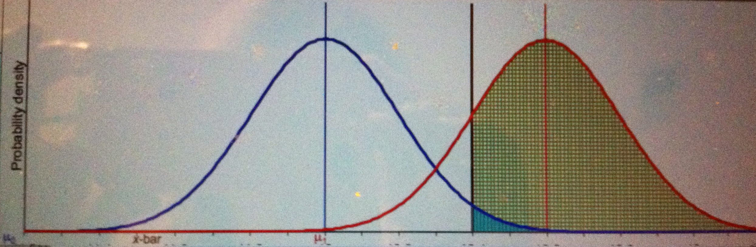
Blue curve is the null, red curve is one possible conjectured alternative: µ = 3. Green area is power, little turquoise area is α.
As Stephen Senn points out (in my favorite of his posts), the alternative against which we set high power is the discrepancy from the null that “we should not like to miss”, delta Δ. Δ is not the discrepancy we may infer from a significant result (in a test where POW(Δ, ) = .84).
So the correct answer is B.
Does A hold true if we happen to know (based on previous severe tests) that µ <µ’? I’ll return to this.
◊Point on language: “to detect alternative µ'” means, “produce a statistically significant result when µ = µ’.” It does not mean we infer µ’. Nor do we know the underlying µ’ after we see the data. Perhaps the strict definition should be employed unless one is clear on this. The power of the test to detect µ’ just refers to the probability the test would produce a result that rings the significance alarm, if the data were generated from a world or experiment where µ = µ’.
[0] A comment by Michael Lew’s brings out my presumption of a given α level, since that is the context in which this matter arises. (I actually have a further destination in mind, indicated in red,, and it won’t be clear until a follow -up). Back to Lew’s query: power is always defined for the “worst case” of just reaching the α level cut-off, which is why I prefer the data-dependent severity, or associated confidence interval. Lew’s reference to a likelihood analysis underscores the need to indicate how one is evaluating evidence. Although I indicated “practicing within the error statistical tribe”, perhaps that was too vague. Still, the interpretation in the case he gives is not very different (except that I wouldn’t favor x over µ’. I thank Lew for his graphic. PastedGraphic-5
[i] I surmise, without claiming a scientific data base, that this fallacy has been increasing over the past few years. It was discussed way back when in Morrison and Henkel (1970). (A relevant post relates to a Jackie Mason comedy routine.) Research was even conducted to figure out how psychologists could be so wrong. Wherever I’ve seen it, it’s due to (explicitly or implicitly) transposing the conditional in a Bayesian use of power. For example, (1 – β)/ α is treated as a kind of likelihood in a Bayesian computation. I say this is unwarranted, even for a Bayesian’s goal, see 2/10/15 post below.
[ii] Pr(M > 2; µ = .25 ) = Pr(Z > 1.75) = .04.
OTHER RELEVANT POSTS ON POWER
- (6/9) U-Phil: Is the Use of Power* Open to a Power Paradox?
- (3/4/14) Power, power everywhere–(it) may not be what you think! [illustration]
- (3/12/14) Get empowered to detect power howlers
- 3/17/14 Stephen Senn: “Delta Force: To what Extent is clinical relevance relevant?”
- (3/19/14) Power taboos: Statue of Liberty, Senn, Neyman, Carnap, Severity
- 12/29/14 To raise the power of a test is to lower (not raise) the “hurdle” for rejecting the null (Ziliac and McCloskey 3 years on)
- 01/03/15 No headache power (for Deirdre)
- 02/10/15 What’s wrong with taking (1 – β)/α, as a likelihood ratio comparing H0 and H1?


")


I haven’t yet encountered A or B, but I often encounter
C. If the test’s power to detect an alternative µ’ to µ is high, then a statistically nonsignificant x is good evidence for µ (or good evidence favoring µ over µ’).
But (as you know) it is easy to construct counterexamples in which P>0.05 yet by all common evidence measures such as likelihood ratios or P-value functions, the evidence favors µ’ over µ.
How would you describe these high-power fallacies in the “tribal” terms you used above?
Hi Sander. Thanks for your comment–I chose between 2 posts on draft, and the other one concerns your question on power analysis for interpreting non-significant results (whereas this post is on interpreting significant results). As you know, since we’ve discussed this,power analysis only allows you to infer there’s evidence for µ is less than µ’ when POW(µ’) is high and the result is not significant. It does not let you infer µ = µo, nor the comparative claim you mention.*
Severity replaces the pre-designated cut-off cα with the observed d0. Thus we obtained the same (but a more custom-tailored) result remaining in the Fisherian tribe, as seen in frequentist Evidential Principle FEV(ii) (in Mayo and Cox 2010):
Click to access Ch%207%20mayo%20&%20cox.pdf
*And don't get me started on shpower analysis (though I'll post on this soon).
some of the notation is garbled in the initial comment, I’ll see what this looks like.
The logic behind A is, I’d think: It’s called power. Power is a good thing, so if a test has low power, everything must be poor, including the evidence we get for a discrepancy in case of significance.
Actually, the setup was presented to me when I was a PhD student by a Bayesian, who knew the right answer, and who used it in order to demonstrate that the frequentists use misleading terminology. (He didn’t win me over, but he had some kind of point.)
Christian: I’m glad to have your comment. But any learning inquiry has to balance things, right? There’s a trade-off between type 1 and 2 error probabilities. (To say the higher the power the lower the type 1 error probability as some (shockingly) do, is to say the two error probabilities go in the same direction.)
High sample size is good, but too high can yield pathologically powerful tests. Robustness is good, but not the coarseness of very low assumptions; we want to find things out but not trivial truths. To me, the idea of very high power goes against the Popperian grain of wanting to block spurious effects and ad hoc saves. Did your teacher say the Bayesians have no trade-offs?
By the way, I deliberately invented severity in such a way that it would always be good (to have passed a severe test). When I first started I didn’t define it that way. Everything else can change, but if you assess severity correctly, swapping out hypotheses as needed, it will always be good.*
*Assuming, that is, the goal of finding things out.
The Bayesian wasn’t a teacher of mine, rather another PhD student whom I met at the time.
Of course you’re right about trade-offs. The trade-off isn’t really in the name, though, in case of power.
Christian: In the name? How would it be in the name? Is it in type 1 error prob? cost? calories? yin? (vs benefit, taste, yang).
Even in ordinary English: absolute power corrupts and all that.
Maybe Fisher’s “sensitivity” works better from the point of view of expressing a trade-off? The fire alarm that is too sensitive, and goes off with a hint of smoke, is going to give many “false alarms”. And of course, those people who are too sensitive and cry in the face of criticism might be ordered out of the lab (a 2015 joke).
Pingback: Distilled News | Data Analytics & R
I’m not sure that you capture the whole story. There are many different considerations that come into play: the value of H0; the value of H’; the sample size; the true effect size; the observed effect size; and the power. In you example you fix the sample size and vary H’, with the result is that option B is correct. However, if you fix both H’ and the observed effect size and obtain the low and high power variants by varying sample size, it seems to be the high power variant (large n) where the evidence in favour of a true effect of at least H’-H0 is strongest, and thus option A is correct.
Michael: Give me numbers and discrepancies to see what happens: n = 25, n = 100 (as in the blog), n = 400. Keep sigma at 10, yielding sigma/root n of 2, 1, .5 . Might as well keep null at 0.
I’d write it out, but I’m madly packing to catch an early plane.
Michael: I hope you discovered that the claim B still holds when you change the sample size. Writing this at the airport, so this might end abruptly. The higher- powered tests are desirable because they are more capable of yielding significant results, but any such a-level result will be indicative of a smaller discrepancy when achieved w/ the higher sample size. In cases where it’s thought the discrepancies (from the null) are small, some say, the high-power inference to a small discrepancy is more in line with the correct value. This assumes B, it does not count against B. It makes use of the fact that error probs take into account sample size (the size of the fishnet, as it were).(Raising the power, shrinks the mesh of the fishnet; the test might only allow the report “I’ve caught a minnow”. That’s as it should be, it’s statistical accounts that do not pick up on sample size that baffle me.)
The significant result with the comparatively lower sample size indicates a greater discrepancy, ASSUMING the error probabilities aren’t spurious! I think the real problem people have with (alleged) significant results with tests considered to have low power to detect the small effects expected in some fields (like social psych) is that they don’t believe the reported error probs are genuine. They suspect they were reached via biasing selection effects and QRPs. But in that case, one cannot rely on the alleged properties of the test to mount an argument about what is or is not warranted. Instead one is voicing a suspicion that the test wasn’t well run. But one can cheat with powerful tests too, so that even a reported (small) discrepancy with a “powerful” test is bogus.
I wrote the above in transit, but it wasn’t sent til now. I will write this up more clearly when I have time over the weekend.
Mayo, you write “The significant result with the comparatively lower sample size indicates a greater discrepancy”, but I wrote that the observed effect size is fixed so we are talking about different cases. The larger sample size will have given a smaller P-value. Are you assuming a fixed P-value? That is not the case I described.
Michael: Keep it fixed and vary whatever you like. Yes I assumed fixed P-value, as that is assumed by those who make the claims in question Please produce numbers so we can see your point.
Where does it say fixed P-value?
Graphs are better than numbers for this type of discussion. I’ve sent a diagram by private email that should serve to explain the issue far better than a couple of numbers can do.
Michael: I added note [0] to indicate that I did have in mind an alpha significant difference. Michael’s point, in relation to a test made powerfully sensitive by dint of sample size,boils down to the fact that ostensibly the “same” Mo value constitutes a larger number of (σ/ √n) units, as n increases. The test or estimate takes into account the sample size as it should.
I gave some numbers to his graph, they are easy to come by.It is true that, say, if n =1600 (in the test T+ defined in the post) that the 2-standard deviation cut-off for rejection becomes .5. (σ/ √n)= 10/40. Call this Test+#2. Let Mo = 1. Test T+#2 will reject and infer µ > 0 (at ~ .025 level) whereas T+#1 will not reject, but will find the result statistically significant at only the .16 level.
But one can’t suppose that Mo = 1 is in front of us, and we get to choose whether to interpret it as if it came from n = 100 or n =1600. Changing the sample size changes what counts as a single sample. Test +#2 is picking up on such small discrepancies that the outcome Mo is 4 standard deviations away from the null of 0.
Yet it’s true that the outcome, were it to come from T+#2, would indicate claims such as µ > .75 with severity (or CI level) .84, and it’s also true that predesignated POW(T+#2,µ = .75) = high (.84), being computed at the worst case of Mo= .5. It’s a rather irrelevant (overly conservative) computation in relation to the given Mo. The “attained” power for µ = .75 is low, 16.
So our analysis agrees with yours. We mainly differ in that (a) the error statistician would reject your likelihood construal, that .5 “is favored” over .75., and (b)we may differ radically in that likelihood favoring doesn’t pick up on biasing selection effects—but let’s assume there are none.
Please correct any errors, I did this quickly.
Thanks Mayo. I have just a few minor follow up comments. First, I think that the reason that I looked at the problem differently from you was your use of ‘significant’ to mean that the P-value = alpha. I did not pick that up. Even though P-values have become ‘personae non-grata’ in some circles, we need them. If you had written that the P-value was the same in all cases then my example would have been clearly out of bounds. We should not trust the word ‘significant’ to communicate any particular meaning.
Second, thank you for linking my diagram. I would like to emphasise that an advantage of the likelihood function over the presentation of the information in your text is that it draws the eye to the location of the actually observed estimate in relationship to the null hypothesis and any other specified hypotheses in the most straightforward way. The entire likelihood function is far more informative than any individual numerical summary, be it a P-value or a likelihood ratio.
Finally, you mention in your final comment (but not the initial statement of problem) the possibility of biassed selection effects and imply that likelihood analyses are especially sensitive to them. They are not. Inferences based on likelihood functions are affected by hidden or unknown selection bias to exactly the same extent as your error statistical approaches are. Known bias can be incorporated into a likelihood-based inference in any way that the analyst feels appropriate, just as a frequentist analyst can arbitrarily choose the model and adjustments for the various aspects of experimental design that affect conditional and unconditional error rates. It is often wrongly assumed (by you as well as others) that a likelihood function (or, worse, a single likelihood ratio) entails an inferential response that precludes incorporation of other types of information. The likelihood function provides a picture of the evidence in the data relevant tot he model parameter of interest: it can support inference but it does not constitute inference. A likelihoodist has no more and no less freedom of arbitrary analytical choices than a frequentist, but does have the advantage of the clarity of expression of the evidence in the data that is provided by the likelihood function.
Michael: It’s interesting that you value seeing the points that “fit” to comparatively different degrees, as given by the likelihood ratios. To me that opens the door to the deepest problem of inductive inference: we can too easily find hypotheses that fit given data, or find data to fit favored hypotheses, and so on. I don’t consider it very useful to know that this is less likely than that, and that is more likely than this–especially when these have small likelihoods. We need to make statistical inferences and this comparative stuff is scarcely more than deductively reporting on likelihoods assuming a model. The inferences in your graphical analysis that do the work are not in the form of a comparative likelihood analysis, but rather a confidence bound.
I think we’ve been through the business of the Likelihood Principle, the Stopping Rule Principle, the irrelevance of the sample space touted by likelihoodists. I don’t know what you mean that you can incorporate them in any way you feel appropriate–but if you mean to say that you will add to your likelihood analysis an assessment of the error probabilistic properties of the overall procedure, then that’s all to the good. But you need principled reasons. The Law ofLikelihood does not provide them.
Royall and others make it clear those considerations are not part of the “evidence’, and you also have argued that way on this blog. So if you’re moving into the error statistical camp, welcome.
Mayo, your point about always being able to find hypotheses that fit the data is way off target, as you will find when you get around to reading my recent paper (http://arxiv.org/abs/1507.08394).
The hypothesis labelled x on my diagram is not an irrelevant hypothesis dreamed up by some perverse analyst, it is the hypothesis pointed to by the evidence. It is on the same scale as the pre-specified (presumably pre-specified) hypotheses H0 and u’, and it is a value of that same model parameter. There is nothing arbitrary about it.
I too, like the interval as the basis of inference. The likelihood function provides the interval that comes from the data in hand relevant to the hypotheses of interest to the analyst given her choice of model. The frequentist confidence interval performs quite well for inference as a consequence of having a similar (same, usually) central point to the likelihood interval.
The likelihood principle refers to evidence, not inference. It is silent about what additional information is available and how to use it. The repeated sampling principle might be interpreted as implying rules for inference, but it is certainly silent about evidence. By assuming, falsely, that the likelihood principle is about inference you are setting too high a bar for utility for the likelihood principle. Again, my recent paper will be helpful (http://arxiv.org/abs/1507.08394).
Michael: Your hypothesis may be pointed to by the evidence, and that is exactly the problem. There are all kinds of hypotheses I can find looking at the data. I didn’t say the hypothesis was irrelevant. Moreover, it’s not enough that you can use a kosher hypothesis, if the account also allows non-kosher ones. The distinction between evidence and inference—something I never heard the likelihoodist try before–sounds like a way to both admit and deny the relevance of error probabilities to the import of the data. You are inventing new things as you go Michael. I’ve written a lot about the likelihood principle, and it’s always been about inference. Royall doesn’t have a 4th category, unless you are putting it under his decision, which surely doesn’t capture inference, as I see it. If the categories were so separate, one might ask why Royall and other likelihoodists are so keep to show how wrong hypotheses testing is for evidence/inference. I’ll be glad to read your paper. Thanks.
Mayo, I know that you have written a lot about the likelihood principle in terms of inference. I usually responded by trying to explain the error (well, more certainly, I tried to explain my interpretation), and quite frequently you simply wrote that I should read older posts on you blog. Now that I’ve loaded the full arguments in the arXived paper, I am prepared to press the issue with you. Why do you think that the likelihood principle refers to inference rather than evidence?
On the topic of your preference for the pre-specified u’ over the data-derived most likely estimate x, would you still prefer u’ if it was outside the 95% confidence interval derived from the data? If not, then how is that consistent with a preference for u’ over x? If so, what does that imply about the interval?
Michael: You can play semantic games fine, but which of the three pigeon holes of Royall do you place inference? I don’t regard inference as distinct from learning or finding things out, so if your LRs are not inference, they might be just data description? If so, then likelihoodists have no grounds to criticize inferential methods with which they disagree: they’re just doing something quite different. And yet all likelihoodists DO criticize other inferential methods with which they disagree. Unlike you, they think they’re providing an account of inference.
On your last para, I never said that and it’s abundantly silly.
Mayo, have a look at the footnote [o] in the main post. You wrote “I wouldn’t favor x over µ’”. I took that to mean that you preferred u’ over x. Forgive me if I have misunderstood.
I do not feel that it is my role to defend Royall. His book is as much polemic as instruction, and I do not agree with all he wrote. In particular he spends a few pages on attacking the evidential interpretation of P-values with irrelevancies and distorted accounts. There are other accounts of likelihood that you should explore. I found Edwards’s book Likelihood to be very useful.
Having said that about Royal, I will add that his depiction of likelihood functions as “what the data say” matches my own view. Formed my view, in fact. If you want to use “inference” in a way that encompasses observing what the data say then I can’t stop you, but I would say that we would then need another word that makes a distinction between observation and what I would mean by inference.
Dear Michael,
I had a quick read of your paper. As I have indicated on this blog I tend to agree with your points – most objections to likelihood analysis seem to rely on degenerate cases (number of parameters > numbers of data points) or an inappropriate generating model/comparison of different generating models. I also find Royall’s presentation to be much weaker than Edwards’ (also: Hacking’s review is not sufficient grounds to reject Edwards approach IMO as I feel it misses crucial points).
In the degenerate cases I feel one has no choice but to either report it as degenerate or introduce additional information to turn an ill-posed problem into a well-posed problem. This later approach is what is done in a) Bayesian statistics with priors, b) inverse problem theory with regularization/additional constraints and c) statistical/machine learning with penalties/regularization (a la Hastie et al.). Multiple applied fields have developed essentially identical mathematical apparatus for dealing with these problems, and I can’t really take philosophical criticism too seriously unless it engages properly with this literature.
Michael: I can’t tell what post this is commenting on. Just one point: It’s impossible to say that the irrelevance of error probabilities (the irrelevance of the sample space, as likelihoodists put it) is an incidental feature of the account to be dealt with by means of priors or penalties. That Royall would have to change the aim to “what you believe” in order to appeal to priors, as he does, in order for you to criticize a best fitting hypothesis is what makes the account inadequate in an inessential way. Moreover, these are not degenerate cases, appealing to max likely hypotheses is the norm and result in inferring hypotheses despite terrible error probabilities, even when they are ordinary parametric hypotheses. That likelihoodists do not have error control is well known (from the LP). Some frequentist accounts do employ penalties in modeling,which is something else.
Incidentally, I happened to come across a new likelihoodist text by Charles Rohde that includes severity.
I cannot see where Option A is ever correct, as worded, and as a general statement. Suppose Ho = 0 and H’ = 5 and effect size is 3, but sample x=-3? Yes, the p-value is lower with large N than it would be with sma!her N, but severity does not favor inferring H’. Quite the opposite.
John: I think this may get to a different, though related, point. In order to keep to “power” (though I’m so used to computing severity), I imagine the observed difference was just significant at the cut-off for which a test’s power is defined. By the way, I find “effect size” is used so equivocally (between an observed difference and a parametric discrepancy) that it’s clearer to call the parametric effect size the “discrepancy” or some other term. I see some people take the observed difference as the inferred discrepancy, and then say it’s an exaggeration of what’s warranted. It is!
Statistically significant should be taken as not understood out of context.
As you often recall, Fisher required regularly being able to generate statistical significance for it to mean anything more than with a single study “Hey guys, we should consider redoing the experiment and see if we regularly get p_values that would unlikely come from a Uniform(0,1) distribution. (Though actually his preferred assessment was combining likelihoods from the individual studies.)
Moreover, whether inference to µ > µ’ is warranted should not be based on just a p_value or even a collection of p_values from replicated studies but all background information bearing on µ.
Language clarification did help, as this is not a common way for statisticians to think about result of a single study (so a useful post). If its a randomized study in clinical medicine, I would be thinking of µ > 0 as involving much less complication and of primary concern than pinning down a particular range of values of µ.
Keith O’Rourke
phan: Naturally, I was taking up an issue “as I find it” as it were, even though I too would want lots of qualifications before inferring a genuine effect. I certainly agree that “isolated” p-values rarely suffice (David Cox gives a taxonomy).
As for
“whether inference to µ > µ’ is warranted should not be based on just a p_value or even a collection of p_values from replicated studies but all background information bearing on µ.”
I think one has to clarify whether one is trying to interpret what the data indicate (from this study or a group of studies, say) and what is warranted given everything we know (your reference to “all background information bearing on µ”)
An example that comes to mind: Given everything we know (e.g., about how severely tested special relativity is), when the OPERA studies appeared to show a violation of the well-known speed of light, scientists wouldn’t dream of averaging in this background with the OPERA results to get a “better estimate” of the warranted speed of light. The background knowledge plays an important role in identifying anomalies and raising suspicions about experimental errors (as in this case). The question of what is warranted, given everything we or I know, might be called “big picture” inference, whereas learning from specific data also has a very important role, especially when we’re striving to get novel truths. We need to distinguish the “level” at which the problem or question lies. I think formal statistics operates at the more local levels of learning from data, even though I am glad to view statistical science more broadly.
Not sure about Fisher and combining likelihoods.
> I think formal statistics operates at the more local levels of learning from data
Conventionally it is – but it shouldn’t be.
I argued this point “Fisher’s key ideas in his theory of statistics … arose from his thinking of statistics as the combination of estimates” here http://andrewgelman.com/wp-content/uploads/2010/06/ThesisReprint.pdf
(Most of it is in the history section and provides numerous direct quotes.)
Given some data, the rejection of the null hypothesis will be completely independent of the alternative chosen. It could be close to the null (the power of the test would be lower) or far from it (the power would be higher). How could the same data and the same rejection outcome give stronger support to the more extreme inference?
Let’s say I want to test if a temperature is higher than 100°F and my thermometer has normal error with standard deviation 1°F. If I make a single measurement, it will be significant (one-sided alpha 0.025) if the reading is above 101.96°F. Is the test powered to reject the null if the actual temperature is 120°F? Absolutely, the power is quite close to 1. Is the test powered to reject the null if the actual temperature is 102°F? Not really, the power is around 0.5. Now, if I make my measurement and announce that it’s significant (i.e. above 101.96°F) I would be quite surprised to find anyone arguing that the evidence for the actual temperature being above 110°F is stronger than the evidence for it being above 102°F. I think even frequentists would notice the logical inconsistency!
Carlos: Well the argument is a frequentist one, relying on error probs being sensitive to sample size, whereas some who practice in alternative tribes have a tendency to argue, in effect, that the higher the power the higher the hurdle for rejection.*
*https://errorstatistics.com/2014/12/29/to-raise-the-power-of-a-test-is-to-lower-the-hurdle-for-rejecting-the-null-ziliac-and-mccloskey-3-years-on/
Carlos: Not sure why you say “even a frequentist” would see the inconsistency when it is an incorrect Inference according to frequentist principles. Rejection of the null in a significance test does not say anything about any particular alternative.
John: It’s just part of the cavalier ridicule to which exiles are put, so I didn’t take it seriously. I don’t know the person commenting.
No offense intended, I was referring only to those confused frequentist practitioners who hold that if POW(µ’) is high then the inference to µ > µ’ is warranted. My argument was just a restatement of the one in the blog post, I find using a concrete example makes the point more clear.
Carlos: Thanks for clarifying. Yes, even those confused about this ought to get it.
Readers: I went back to reread the discussion after Senn’s Delta Force post*,and even added a comment:
https://errorstatistics.com/2014/03/17/stephen-senn-on-how-to-interpret-discrepancies-against-which-a-test-has-high-power-guest-post/comment-page-1/#comment-128573
I understand better now what Senn was saying about the alternative “you don’t want to miss”. Of course this is determined by all kinds of things and it’s a “planning parameter” as he says. I wonder, just wrt this one point, how typical the drug testing situation is in science more generally. For example, in searching for the Higgs particle, high energy physicists (HEPs) were hoping to find a much larger particle (in terms of energy levels) than they did, but they didn’t want to miss any particle at any energy level. That is, they want to find out its properties, whatever they are. Anyway, I would like to recommend people have a look at:
https://errorstatistics.com/2014/03/17/stephen-senn-on-how-to-interpret-discrepancies-against-which-a-test-has-high-power-guest-post/
https://errorstatistics.com/2014/03/17/stephen-senn-on-how-to-interpret-discrepancies-against-which-a-test-has-high-power-guest-post/#comment-25609
*Which I thought sounded too “star warsy”, but he wasn’t keen on my substitute, whatever it was.