Capability and Severity: Deeper Concepts: Excerpts From Excursion 3 Tour III

Deeper Concepts 3.7, 3.8

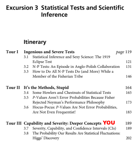
Tour III Capability and Severity: Deeper Concepts

From the itinerary: A long-standing family feud among frequentists is between hypotheses tests and confidence intervals (CIs), but in fact there’s a clear duality between the two. The dual mission of the first stop (Section 3.7) of this tour is to illuminate both CIs and severity by means of this duality. A key idea is arguing from the capabilities of methods to what may be inferred. The severity analysis seamlessly blends testing and estimation. A typical inquiry first tests for the existence of a genuine effect and then estimates magnitudes of discrepancies, or inquires if theoretical parameter values are contained within a confidence interval. At the second stop (Section 3.8) we reopen a highly controversial matter of interpretation that is often taken as settled. It relates to statistics and the discovery of the Higgs particle – displayed in a recently opened gallery on the “Statistical Inference in Theory Testing” level of today’s museum.

3.7 Severity, Capability, and Confidence Intervals (CIs)

It was shortly before Egon offered him a faculty position at University College starting 1934 that Neyman gave a paper at the Royal Statistical Society (RSS) which included a portion on confidence intervals, intending to generalize Fisher’s fiducial intervals. With K. Pearson retired (he’s still editing Biometrika but across campus with his assistant Florence David), the tension is between E. Pearson, along with remnants of K.P.’s assistants, and Fisher on the second and third floors, respectively. Egon hoped Neyman’s coming on board would melt some of the ice.

Neyman’s opinion was that “Fisher’s work was not really understood by many statisticians . . . mainly due to Fisher’s very condensed form of explaining his ideas” (C. Reid 1998, p. 115). Neyman sees himself as championing Fisher’s goals by means of an approach that gets around these expository obstacles. So Neyman presents his first paper to the Royal Statistical Society (June, 1934), which includes a discussion of confidence intervals, and, as usual, comments (later published) follow. Arthur Bowley (1934), a curmudgeon on the K.P. side of the aisle, rose to thank the speaker. Rubbing his hands together in gleeful anticipation of a blow against Neyman by Fisher, he declares: “I am very glad Professor Fisher is present, as it is his work that Dr Neyman has accepted and incorporated. . .  I am not at all sure that the ‘confidence’ is not a confidence trick” (p.132). Bowley was to be disappointed. When it was Fisher’s turn, he was full of praise. “Dr Neyman . . . claimed to have generalized the argument of fiducial probability, and he had every reason to be proud of the line of argument he had developed for its perfect clarity” (Fisher 1934c, p.138). Caveats were to come later (Section 5.7). For now, Egon was relieved:

Fisher had on the whole approved of what Neyman had said. If the impetuous Pole had not been able to make peace between the second and third floors of University College, he had managed at least to maintain a friendly foot on each! (C. Reid 1998, p. 119)

 

CIs, Tests, and Severity. I’m always mystified when people say they find P-values utterly perplexing while they regularly consume polling results in terms of confidence limits. You could substitute one for the other. (SIST p. 190)

…

Not only is there a duality between confidence interval estimation and tests, they were developed by Jerzy Neyman at the same time he was developing tests! The 1934 paper in the opening to this tour builds on Fisher’s fiducial intervals dated in 1930, but he’d been lecturing on it in Warsaw for a few years already. Providing upper and lower confidence limits shows the range of plausible values for the parameter and avoids an “ up/down” dichotomous tendency of some users of tests. Yet, for some reason, CIs are still often used in a dichotomous manner: rejecting μ values excluded from the interval, accepting (as plausible or the like) those included. There’ s the tendency, as well, to fix the confidence level at a single 1 − α , usually 0.9, 0.95, or 0.99. Finally, there’ s the adherence to a performance rationale: the estimation method will cover the true θ 95% of the time in a series of uses. We will want a much more nuanced, inferential construal of CIs. We take some first steps toward remedying these shortcomings by relating confidence limits to tests and to severity.

(A) The proofs of Excursion 3 Tour III are here. You can also find many discussions in this blog on confidence intervals (search CIs). Of most relevance to Section 3.7 is a post Duality: Confidence intervals and the severity of tests. Another is Do CIs Avoid Fallacies of Tests? Reforming the Reformers.

……

Live Exhibit (ix). What Should We Say When Severity Is Not Calculable? (SIST p. 200)

In developing a system like severity, at times a conventional decision must be made. However, the reader can choose a different path and still work within this system.

What if the test or interval estimation procedure does not pass the audit? Consider for the moment that there has been optional stopping, or cherry picking, or multiple testing. Where these selection effects are well understood, we may adjust the error probabilities so that they do pass the audit. But what if the moves are so tortuous that we can’t reliably make the adjustment? Or perhaps we don’t feel secure enough in the assumptions? Should the severity for μ > µ₀ be low or undefined?

You are free to choose either. The severe tester says SEV(μ > µ₀) is low. As she sees it, having evidence requires a minimum threshold for severity, even without setting a precise number. If it’s close to 0.5, it’s quite awful. But if it cannot be computed, it’s also awful, since the onus on the researcher is to satisfy the minimal requirement for evidence. I’ll follow her: If we cannot compute the severity even approximately (which is all we care about), I’ll say it’s low, along with an explanation as to why: It’s low because we don’t have a clue how to compute it!

A probabilist, working with a single “probability pie” as it were, would take a low probability for H as giving a high probability to ~H. By contrast we wish to clearly distinguish between having poor evidence for H and having good evidence for ~H. Our way of dealing with bad evidence, no test (BENT) allows us to do that. Both SEV(H) and SEV(~H) can be low enough to be considered lousy, even when both are computable.

…

3.8 The Probability Our Results Are Statistical Fluctuations: the Higgs Discovery (SIST p. 202)

[B] Elements of Section 3.8, in early formulations, may be found in the several posts on the Higgs discovery on this blog. One with links to several parts is Higgs Discovery three years on (Higgs analysis and statistical flukes). Even if you have the book, you might find the valuable comments by readers (made to the original posts) worth checking out.

Where you are in the journey.