Stephen Senn: Being Just about Adjustment (Guest Post)

.

Stephen Senn
Consultant Statistician
Edinburgh

Correcting errors about corrected estimates

Randomised clinical trials are a powerful tool for investigating the effects of treatments. Given appropriate design, conduct and analysis they can deliver good estimates of effects. The key feature is concurrent control. Without concurrent control, randomisation is impossible. Randomisation is necessary, although not sufficient, for effective blinding. It also is an appropriate way to deal with unmeasured predictors, that is to say suspected but unobserved factors that might also affect outcome. It does this by ensuring that, in the absence of any treatment effect, the expected value of variation between and within groups is the same. Furthermore, probabilities regarding the relative variation can be delivered and this is what is necessary for valid inference.

There are two extreme positions regarding randomisation that are unreasonable. The first is that because randomisation only ensures performance in terms of probabilities, it is irrelevant to any actual study conducted. The second is that because randomisation delivers valid estimates on average, using observed covariate information, say in a so-called analysis of covariance (ANCOVA), is unnecessary and possibly even harmful. The first is easily answered, even if many find the answer difficult to understand: probabilities are what we have to use when we don’t have certainties. For further discussion of this see my previous blogs on this site  Randomisation Ratios and Rationality and Indefinite Irrelevance and also a further blog Stop Obsessing about Balance. The second criticism is also, in principle, easy to answer: covariates provide the means of recognising that averages are not relevant to the case in hand (Senn, S. J., 2019). Nevertheless, many trialists stubbornly refuse to use covariate information. This is wrong and in this blog I shall explain why.

Ringing the changes

A variant of the refusal to use covariates occurs when the covariate is a baseline. The argument is then sometimes used that an obviously appropriate ‘response’ variable is the so-called change-score (or gain- score), that is to say, the difference between the variable of interest at outcome and its value at baseline. For example, in a trial of asthma, we might be interested in the variable forced expiratory volume in one second (FEV₁), a measure of lung function. We measure this at outcome and also at baseline and then use the difference (outcome – baseline) as the ‘response’ measure in subsequent analysis.

The argument then continues that since one has adjusted for the baseline, by subtracting it from the outcome, no further adjustment is necessary and furthermore, that analysis of these change-scores being simpler than ANCOVA, it is more robust and reliable.

I shall now explain why this is wrong.

Concentrating on that which is caused

The important point to grasp from the beginning is that what are affected by the treatment are the outcomes. The baselines are not affected by treatment and so they do not carry the causal message. They may be predictive of the outcome, and that being so they may usefully be incorporated in an estimate of the effect of treatment, but treatment only has the capacity to affect the outcomes.

I stress this because much unnecessary complication is introduced by regarding the effect that treatments have on change over time as being fundamental. Such effects on change are a consequence of the effect on outcome: outcome is primary, change is secondary.

Algebra, alas

It will be easier to discuss all this with the help of some symbols. Table 1 shows symbols that can be used for referring to statistics for a parallel group trial in asthma with two arms, control and treatment. To simplify things, I shall take the case where the number of patients in each arm is identical, although this is not necessary to anything important that follows.

A further table, Table 2 gives symbols for various parameters. Some simplifying assumptions will be made that various parameter values do not change from control group to treatment group. For the assumptions in lines 2 and 4, this must be true if randomisation is carried out, since we are talking about expectations over all randomisations and the parameters refer to quantities measured before treatment starts. For lines 3 and 5, the assumptions are true under the null hypothesis that there is no difference between treatment and control.

Starting at the end

Since the treatments can only affect the outcomes, the logical place to start is at the end. Thus, to use a term much in vogue, our estimand (that which we wish to estimate) is  δ = μ_Yt-μ_Yc , the difference in ‘true’ means at outcome. Note that we could define the estimand in terms of the double difference

that is to say the differences between groups of the differences from baseline, but this is pointless because in a randomised trial we have μ_Xc=μ_Xt = μ_X and so this reduces to what we had previously. In fact, if we think of the logic of the randomised clinical trial, by which the patients given control are there purely to estimate what would have happened to the patients given the treatment had they been given the control, this is quite unnecessary.

As a first stab at estimating the estimand, the simplest thing to use is the corresponding difference in statistics, that is to say

This estimator is unbiased for δ: on average it will be equal to the parameter it is supposed to estimate. Its variance, given our assumptions, will be equal to


However, it is not independent of the observed difference at baseline. In fact, given our simplification, it has a covariance with this difference of

where ρ is the correlation between baseline and outcome.

This dependence implies two things. First, it means that although is unbiased, it is not conditionally unbiased. Given an observed difference at baseline,  

we can do better than just assuming that the difference we would see at outcome, in the absence of any treatment effect, would be zero. Zero is the value we would see over all randomisations but it is not the value we would see for all randomised clinical trials with the observed baseline. This can be easily illustrated using a simulation described below.

A simulating discussion

I simulated 1000 clinical trials of a bronchodilator in asthma using forced expiratory volume in one second (FEV₁) as an outcome with parameters set as in Table 3:

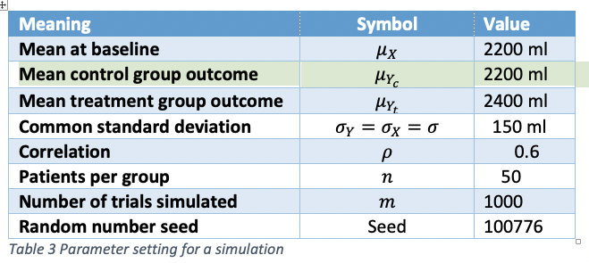
The seed is of no relevance to anybody except me but is included here should I ever need to check back in the future. The other parameters are supposed to be what might be plausible in a such a clinical trial. The values are drawn from a bivariate Normal assumed to be a suitable approximate theoretical model for a randomised clinical trial.

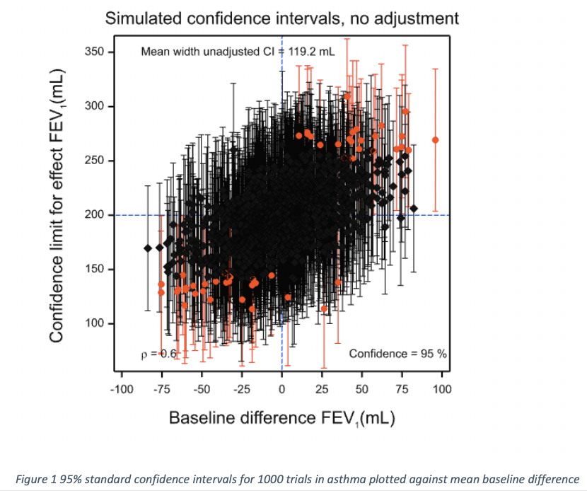
One thousand confidence intervals are displayed in Figure 1. They have been plotted against the baseline difference. Those that are plotted in black cover the ‘true’ value of 200 mL and those that are plotted in red do not. The point estimate is shown by a black diamond in the former case and by a red circle in the latter. There are 949, or 94.9% that cover the true value and 51 or 5.1% that do not. The differences from the theoretical expectations of 95% and 5% are immaterial.

However, since we have baseline information available, we can recognise something about the intervals: where the baseline difference is negative, they are more likely to underestimate the true value and where the difference is positive, they are likely to overestimate it. In fact, generally, the bigger the baseline difference, the worse the coverage. In the view of many statisticians, including me, this means that a confidence interval calculated in this way is satisfactory if the baselines have not been observed but not if they have.

Can we fix this using the change-score? The answer is no. Figure 2 shows the corresponding plot for the change-score. Now we have the reverse problem. Where the baseline difference is negative, the treatment effect is overestimated and where the difference is positive, underestimated. There are exceptions but a general pattern is visible: the estimates are negatively correlated with the baseline difference.

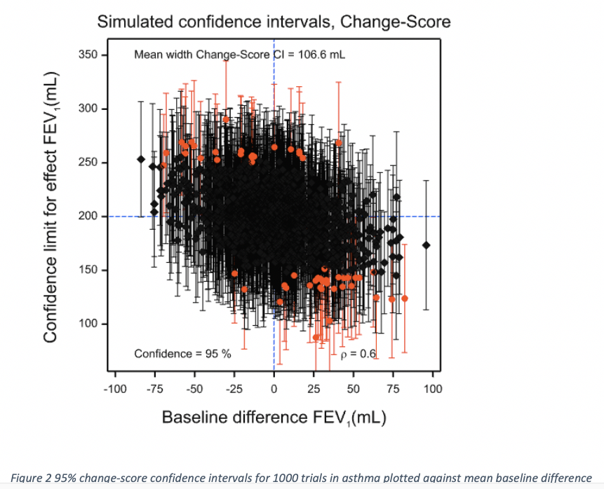
The reason that this happens is that the values are not perfectly predictive of the values at outcome. The way to deal with this is to calculate exactly how predictive the values are using the data within the treatment groups. Because I am in the privileged position of having set the values of the simulation, I know that the relevant slope parameter, β, is 0.6, considerably less than the implicit change-score value of 1. This is because the correlation, ρ was set to be 0.6 and the variances at baseline and outcome were set to be equal. However, I did not ‘cheat’ by using this knowledge to do the adjusted calculation, since in practice I would never know the true value. In fact, for each simulation, the value was estimated from the covariances and variances within the treatment groups.

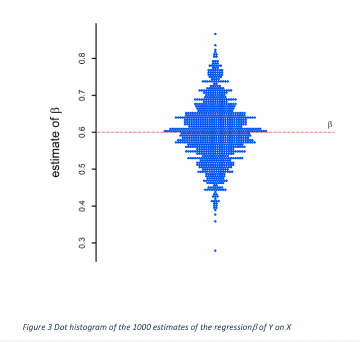
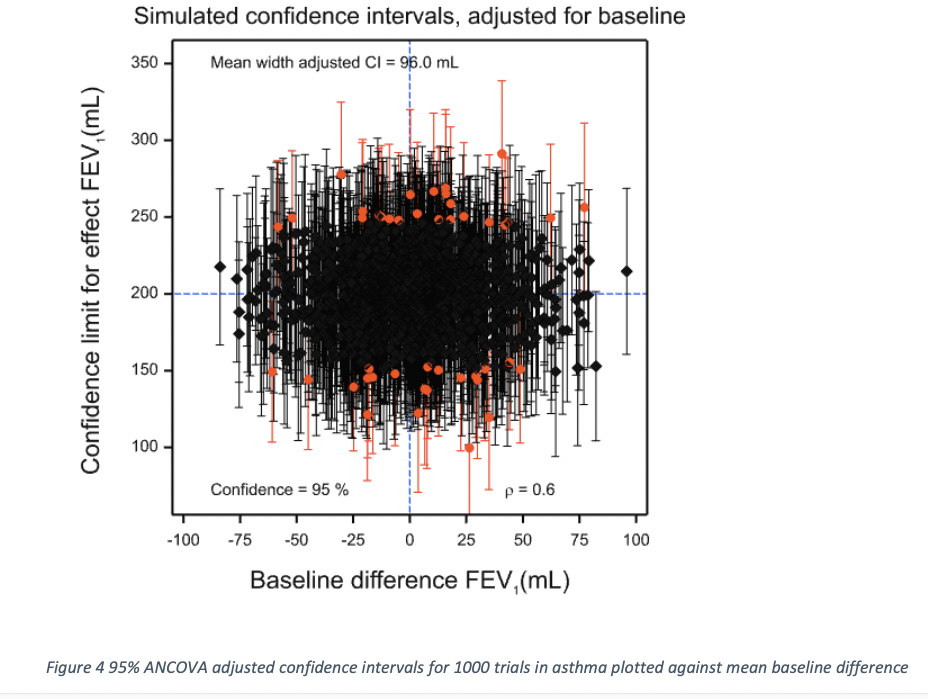
Figure 3 gives a dot histogram for the estimates of β. The mean over the 1000 simulations was 0.601 and the lowest value of the 1000 was 0.279, with the maximum being 0.869. Different values will have been used for different simulated clinical trials to adjust the difference at outcome by the difference at baseline. The adjusted estimates and confidence limits are given in Figure 4 and now it can be seen that these are independent of the baseline differences, which cannot now be used to select which confidence intervals are less likely to include the true value.

Algebra again, alas

The three estimators we have considered can be regarded as a special case of

If we set  b = 0 we have the simple unadjusted estimate of Figure 1. If we set  b = 1 we have the change-score estimate of Figure 2. Finally if we set b = , the within group regression coefficient of Y on X shown in Figure 3, we get the ANCOVA estimate of Figure 4.

Given our assumptions, not unreasonable given the design, we have that the regression of the mean difference at outcome on the mean difference at baseline should be the same as the within groups regression of the individual outcome values. Note that this assumption is not so reasonable for different designs, for example, cluster randomised designs, a point that has been misunderstood in some treatments of Lord’s paradox. See Rothamsted Statistics meets Lord’s Paradox for an explanation and also Red Herrings and the Art of Cause Fishing. Thus, we can now study exactly what is going on in terms of the adjusted within group differences Y – bX. If these adjusted differences are averaged for each of the two groups and we then form the difference of these averages, treatment minus control, we have the estimate  .

Now, the covariance of (Y – bX) & X  is σ_XY – bσ_Xσ_X from which it follows immediately that this is 0 if and only if

Thus, the value of b is then the within-slope regression β, so this is nothing other than the ANCOVA solution. (In practice we have to estimate β, a point to which I shall return later.) Hence, the lack of dependence between estimate and baseline difference exhibited by Figure 4. Note also that dimensional analysis shows that the units of β are units of Y over units of X. In our particular example of using a baseline, these two units are the same and so cancel out but the argument is also valid for any predictor, including one whose units are quite different. Once the slope has been multiplied by an X it yields a prediction in units of Y which is, of course, exactly what is needed for ‘correcting’ an observed Y. This, in my opinion, is yet another argument against the change-score ‘solution’. It only works in a special case for which there is no need to abandon the solution that works generally.

In fact, the change-score works badly. To see this, consider a re-writing of the adjusted outcome as

On the RHS for the first term in square brackets we have the ANCOVA estimate. On the RHS for the second term in square brackets, we have the amount by which any general estimate differs from the ANCOVA estimate. If we calculate the variance of the RHS, we find it consists of three terms. The first of these is the variance of the ANCOVA estimator. The second is (β – b)² times . The third is 2(β – b) times the covariance of [Y – βX] and X. However, we have shown that this covariance is zero. Thus, the third term is zero. Furthermore, the second term, being a product of squared quantities is greater than zero unless β = b but when this is the case we have the ANCOVA solution. Thus, ANCOVA is the minimum variance solution. The change-score solution will have a higher variance.

Simulating summary

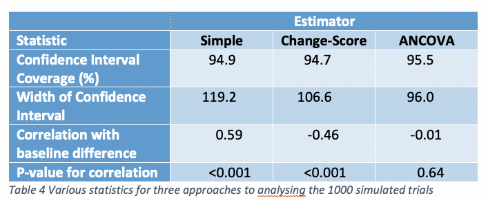
Some summary statistics (over the 1000 simulated trials) are given for the three approaches used to analyse the results. There are no differences worth noticing between coverage. This is because each method of analysis is designed to provide correct coverage on average. The simple analysis of outcomes is positively and highly significantly correlated with the baseline difference. The change-score is highly significantly negatively correlated. The correlation is less in absolute terms because the correlation coefficient used for the simulation (0.6) is greater than 0.5. Had it been less than 0.5, the absolute correlation would have been greater for the change-score. Similarly, although the mean width of the change-score is less than that for the simple analysis, this does not have to be so and is a result of the correlation being greater than 0.5. The ANCOVA estimates are more precise than either and this has to be so in expectation barring a minor issue, discussed in the next section.

A qualifying quibble

It is not quite the case that ANCOVA is the best one can do, since I have assumed in the algebraic development (although not in the simulation) that the slope parameter is known. In practice it has to be estimated and this leads to a small loss in precision compared to the (unrealistic) situation where the parameter is known. Basically, there are two losses: first the degrees of freedom for estimating the error variance are reduced by one and second there is, in practice, a small penalty for the loss of orthogonality. Further discussing of this is beyond the cope of this note but is covered in (Lesaffre, E. & Senn, S., 2003) and (Senn, S. J., 2011). In practice, the effect is small once one has even a modest number of patients.

In conclusion

For randomised clinical trials, there is no excuse for using a change-score approach, rather than analysis of covariance. To do so betrays not only a conceptual confusion about causality but is inefficient. Given the stakes, this is unacceptable (Senn, S. J., 2005).

References

Lesaffre, E., & Senn, S. (2003). A note on non-parametric ANCOVA for covariate adjustment in randomized clinical trials. Statistics in Medicine, 22(23), 3583-3596.

Senn, S. J. (2005). An unreasonable prejudice against modelling? Pharmaceutical statistics, 4, 87-89.

Senn, S. J. (2011). Modelling in drug development. In M. Christie, A. Cliffe, A. P. Dawid, & S. J. Senn (Eds.), Simplicity Complexity and Modelling (pp. 35-49). Chichester: Wiley.

Senn, S. J. (2019). The well-adjusted statistician. Applied Clinical Trials, 2.