Misspecification Testing: (part 2) A Fallacy of Error “Fixing”

Part 1 is here.

Graphing t-plots (This is my first experiment with blogging data plots, they have been blown up a bit, so hopefully they are now sufficiently readable).

Here are two plots (t-plots) of the observed data where y_t is the population of the USA in millions, and  x_t our “secret” variable, to be revealed later on, both over time (1955-1989).

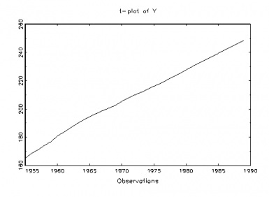
Fig 1: USA Population (y)

Fig. 2: Secret variable (x)

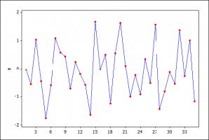
Figure 3: A typical realization of a NIID process.

Pretty clearly, there are glaring departures from IID when we compare a typical realization of a NIID process,  in fig. 3, with the t-plots of the two series  in figures 1-2.  In particular, both data series show the mean is increasing with time – that is, strong mean-heterogeneity (trending mean).Our recommended next step would be to continue exploring the probabilistic structure of the data in figures 1 and 2  with a view toward thoroughly assessing the validity of the LRM assumptions [1]-[5] (table 1). But first let us take a quick look at the traditional approach for testing assumptions, focusing just on assumption [4] traditionally viewed as error non-autocorrelation: E(u_t,u_s)=0 for t≠s, t,s=1,2,…,n.Testing Non-Autocorrelation: The Parametric Durbin-Watson (D-W) Test

The most widely used parametric test for independence is the Durbin-Watson (DW) test.  Here, all the assumptions of the LRM are retained, except the one under test —independence—which is ‘relaxed’.  In particular, the original error term in M₀ is extended to allow for the possibility that the errors u_t are correlated with their own past using a particular form of error correlation known as first order AutoRegression (AR(1)), i.e.

                                    u_t  =ρu_t-1 + ε_t,   t=1,2,…,n,…,

where {ε_t, t=1,2, …, n, …,}  is a Normal, white-noise process.

That is, a new model, the Autocorrelation-Corrected (A-C) LRM, is assumed as the overarching model:

M₁:      y_t = β₀ + β₁x_t + u_t,    u_t  =ρu_t-1 + ε_t,    t=1,2,…,n,…

If ρ = 0, we are back to Ho.  So the D-W test assesses whether or not ρ = 0 in model M₁.  Obviously, either ρ=0 or ρ ≠ 0, but it is a mistake to suppose we are exhausting all possibilities here, unless we are within M₁.  One way to bring this out is to view the D-W test as actually considering the conjunctions:                       

H₀: {M₁ & ρ=0}, vs.  H₁: {M₁ & ρ ≠ 0}.

With the data in our example, the D-W test statistic rejects the null hypothesis (at level .02), which is standardly taken as grounds to adopt H₁. This move to infer H_1, however, is warranted only if we are within M₁. True, if ρ = 0, we are back to the LRM, but ρ ≠ 0 does not entail the particular violation of independence asserted in H₁. Nevertheless, modelers routinely go on to infer H₁ upon rejecting H₀, despite warnings, e.g., “A simple message for autocorrelation correctors: Don’t” (Mizon, 1995). 

But it must be admitted that such warnings, right-headed as they are, generally do not go hand in hand with a clear elucidation of why the reasoning is flawed. Only with such an elucidation can one grasp the fallacy that prevents this strategy from uncovering what is really wrong, both with the original LRM and the autocorrelation-corrected (A-C) version of LRM. The latter may be written as A-C LRM, which is too many letters, but not too bad.

Granted, the flaw is not entirely obvious at first, and so it is perhaps understandable that, far from detecting the fallacy, the traditional strategy finds strong evidence that the data misfit makes it necessary to infer the error-autocorrelation of the new model.

 Having inferred the A-C LRM, the traditional strategy goes merrily on its way  to estimate the new model yielding:

M₁:      y_t = 167.2+ 1.9x_t + û_t,  u_{t =} .43u_t-1 + ε_t,      
It appears that the A-C LRM has ‘corrected for’ the anomalous result that led to rejecting the LRM–at least according to the traditional analysis. After all, if we go on to check if the new error process {ε_t, t=1,2, …, n, …,}  is free of any autocorrelation by running another DW test–as is the common strategy– we find indeed it is[1].

Although the A-C LRM has, in one sense, ‘corrected for’ the presence of autocorrelation, because the assumptions of model M₁ have been retained in H₁, this check had no chance to uncover the various other forms of dependence that could have been responsible for ρ ≠  0. Thus the inference to H₁ lacks severity.

Duhemian problems loom large.  By focusing exclusively on the error term the traditional viewpoint overlooks the ways the systematic component of M₁ may be misspecified and fails also to acknowledge other hidden assumptions, e.g.,

θ:=(β₀ , β₁, σ²), are not changing with the index  t =1, 2, …, n.

These logical failings lead to a model which, while acceptable according to its own self-scrutiny, is in fact statistically inadequate. If used for the ‘primary’ statistical inferences, the actual error probabilities are much higher than the ones it is thought to license, and such inferences are unreliable at predicting  values beyond the data used.  This  illustrates the kind of pejorative use of the data to construct (ad hoc) a model to account for an anomaly that leads many philosophers of science, as well as statistical modelers, to be wary of any and all misspecification, since ‘double counting’ is involved. But it is a mistake to lump all m-s tests together in the same bin. What is a better way?  Stay tuned!

 See other parts:

PART 3: https://errorstatistics.com/2012/02/27/misspecification-testing-part-3-m-s-blog/

PART 4: https://errorstatistics.com/2012/02/28/m-s-tests-part-4-the-end-of-the-story-and-some-conclusions/

PART 1: https://errorstatistics.com/2012/02/22/2294/