Posts Tagged With: Aris Spanos

A. Spanos: Egon Pearson’s Neglected Contributions to Statistics

egon pearson swim

11 August 1895 – 12 June 1980

Today is Egon Pearson’s birthday. I reblog a post by my colleague Aris Spanos from (8/18/12): “Egon Pearson’s Neglected Contributions to Statistics.”  Happy Birthday Egon Pearson!

    Egon Pearson (11 August 1895 – 12 June 1980), is widely known today for his contribution in recasting of Fisher’s significance testing into the Neyman-Pearson (1933) theory of hypothesis testing. Occasionally, he is also credited with contributions in promoting statistical methods in industry and in the history of modern statistics; see Bartlett (1981). What is rarely mentioned is Egon’s early pioneering work on:

(i) specification: the need to state explicitly the inductive premises of one’s inferences,

(ii) robustness: evaluating the ‘sensitivity’ of inferential procedures to departures from the Normality assumption, as well as

(iii) Mis-Specification (M-S) testing: probing for potential departures from the Normality  assumption.

Arguably, modern frequentist inference began with the development of various finite sample inference procedures, initially by William Gosset (1908) [of the Student’s t fame] and then Fisher (1915, 1921, 1922a-b). These inference procedures revolved around a particular statistical model, known today as the simple Normal model: Continue reading

Categories: phil/history of stat, Statistics, Testing Assumptions | Tags: , , ,

Phil 6334: Misspecification Testing: Ordering From A Full Diagnostic Menu (part 1)

.

 We’re going to be discussing the philosophy of m-s testing today in our seminar, so I’m reblogging this from Feb. 2012. I’ve linked the 3 follow-ups below. Check the original posts for some good discussion. (Note visitor*)

“This is the kind of cure that kills the patient!”

is the line of Aris Spanos that I most remember from when I first heard him talk about testing assumptions of, and respecifying, statistical models in 1999.  (The patient, of course, is the statistical model.) On finishing my book, EGEK 1996, I had been keen to fill its central gaps one of which was fleshing out a crucial piece of the error-statistical framework of learning from error: How to validate the assumptions of statistical models. But the whole problem turned out to be far more philosophically—not to mention technically—challenging than I imagined. I will try (in 3 short posts) to sketch a procedure that I think puts the entire process of model validation on a sound logical footing. Continue reading

Categories: Intro MS Testing, Statistics | Tags: , , , ,

More on deconstructing Larry Wasserman (Aris Spanos)

This follows up on yesterday’s deconstruction:


 Aris Spanos (2012)[i] – Comments on: L. Wasserman “Low Assumptions, High Dimensions (2011)*

I’m happy to play devil’s advocate in commenting on Larry’s very interesting and provocative (in a good way) paper on ‘how recent developments in statistical modeling and inference have [a] changed the intended scope of data analysis, and [b] raised new foundational issues that rendered the ‘older’ foundational problems more or less irrelevant’.

The new intended scope, ‘low assumptions, high dimensions’, is delimited by three characteristics:

“1. The number of parameters is larger than the number of data points.

2. Data can be numbers, images, text, video, manifolds, geometric objects, etc.

3. The model is always wrong. We use models, and they lead to useful insights but the parameters in the model are not meaningful.” (p. 1)

In the discussion that follows I focus almost exclusively on the ‘low assumptions’ component of the new paradigm. The discussion by David F. Hendry (2011), “Empirical Economic Model Discovery and Theory Evaluation,” RMM, 2: 115-145,  is particularly relevant to some of the issues raised by the ‘high dimensions’ component in a way that complements the discussion that follows.

My immediate reaction to the demarcation based on 1-3 is that the new intended scope, although interesting in itself, excludes the overwhelming majority of scientific fields where restriction 3 seems unduly limiting. In my own field of economics the substantive information comes primarily in the form of substantively specified mechanisms (structural models), accompanied with theory-restricted and substantively meaningful parameters.

In addition, I consider the assertion “the model is always wrong” an unhelpful truism when ‘wrong’ is used in the sense that “the model is not an exact picture of the ‘reality’ it aims to capture”. Worse, if ‘wrong’ refers to ‘the data in question could not have been generated by the assumed model’, then any inference based on such a model will be dubious at best! Continue reading

Categories: Philosophy of Statistics, Spanos, Statistics, U-Phil, Wasserman | Tags: , , , ,

A. Spanos: Egon Pearson’s Neglected Contributions to Statistics

may-4-8-aris-spanos-e2809contology-methodology-in-statistical-modelinge2809dWith permission from my colleague Aris Spanos, I reblog his (8/18/12): “Egon Pearson’s Neglected Contributions to Statistics“. It illuminates a different area of E.S.P’s work than my posts here and here.

    Egon Pearson (11 August 1895 – 12 June 1980), is widely known today for his contribution in recasting of Fisher’s significance testing into the Neyman-Pearson (1933) theory of hypothesis testing. Occasionally, he is also credited with contributions in promoting statistical methods in industry and in the history of modern statistics; see Bartlett (1981). What is rarely mentioned is Egon’s early pioneering work on:

(i) specification: the need to state explicitly the inductive premises of one’s inferences,

(ii) robustness: evaluating the ‘sensitivity’ of inferential procedures to departures from the Normality assumption, as well as

(iii) Mis-Specification (M-S) testing: probing for potential departures from the Normality  assumption.

Arguably, modern frequentist inference began with the development of various finite sample inference procedures, initially by William Gosset (1908) [of the Student’s t fame] and then Fisher (1915, 1921, 1922a-b). These inference procedures revolved around a particular statistical model, known today as the simple Normal model:

Xk ∽ NIID(μ,σ²), k=1,2,…,n,…             (1)

where ‘NIID(μ,σ²)’ stands for ‘Normal, Independent and Identically Distributed with mean μ and variance σ²’. These procedures include the ‘optimal’ estimators of μ and σ², Xbar and s², and the pivotal quantities:

(a) τ(X) =[√n(Xbar- μ)/s] ∽ St(n-1),  (2)

(b) v(X) =[(n-1)s²/σ²] ∽ χ²(n-1),        (3)

where St(n-1) and χ²(n-1) denote the Student’s t and chi-square distributions with (n-1) degrees of freedom.

The question of ‘how these inferential results might be affected when the Normality assumption is false’ was originally raised by Gosset in a letter to Fisher in 1923:

“What I should like you to do is to find a solution for some other population than a normal one.”  (Lehmann, 1999)

He went on to say that he tried the rectangular (uniform) distribution but made no progress, and he was seeking Fisher’s help in tackling this ‘robustness/sensitivity’ problem. In his reply that was unfortunately lost, Fisher must have derived the sampling distribution of τ(X), assuming some skewed distribution (possibly log-Normal). We know this from Gosset’s reply:

“I like the result for z [τ(X)] in the case of that horrible curve you are so fond of. I take it that in skew curves the distribution of z is skew in the opposite direction.”  (Lehmann, 1999)

After this exchange Fisher was not particularly receptive to Gosset’s requests to address the problem of working out the implications of non-Normality for the Normal-based inference procedures; t, chi-square and F tests.

In contrast, Egon Pearson shared Gosset’s concerns about the robustness of Normal-based inference results (a)-(b) to non-Normality, and made an attempt to address the problem in a series of papers in the late 1920s and early 1930s. This line of research for Pearson began with a review of Fisher’s 2nd edition of the 1925 book, published in Nature, and dated June 8th, 1929.  Pearson, after praising the book for its path breaking contributions, dared raise a mild criticism relating to (i)-(ii) above:

“There is one criticism, however, which must be made from the statistical point of view. A large number of tests are developed upon the assumption that the population sampled is of ‘normal’ form. That this is the case may be gathered from a very careful reading of the text, but the point is not sufficiently emphasised. It does not appear reasonable to lay stress on the ‘exactness’ of tests, when no means whatever are given of appreciating how rapidly they become inexact as the population samples diverge from normality.” (Pearson, 1929a)

Fisher reacted badly to this criticism and was preparing an acerbic reply to the ‘young pretender’ when Gosset jumped into the fray with his own letter in Nature, dated July 20th, in an obvious attempt to moderate the ensuing fight. Gosset succeeded in tempering Fisher’s reply, dated August 17th, forcing him to provide a less acerbic reply, but instead of addressing the ‘robustness/sensitivity’ issue, he focused primarily on Gosset’s call to address ‘the problem of what sort of modification of my tables for the analysis of variance would be required to adapt that process to non-normal distributions’. He described that as a hopeless task. This is an example of Fisher’s genious when cornered by an insightful argument. He sidestepped the issue of ‘robustness’ to departures from Normality, by broadening it – alluding to other possible departures from the ID assumption – and rendering it a hopeless task, by focusing on the call to ‘modify’ the statistical tables for all possible non-Normal distributions; there is an infinity of potential modifications!

Egon Pearson recognized the importance of stating explicitly the inductive premises upon which the inference results are based, and pressed ahead with exploring the robustness issue using several non-Normal distributions within the Pearson family. His probing was based primarily on simulation, relying on tables of pseudo-random numbers; see Pearson and Adyanthaya (1928, 1929), Pearson (1929b, 1931). His broad conclusions were that the t-test:

τ0(X)=|[√n(X-bar- μ0)/s]|, C1:={x: τ0(x) > cα},    (4)

for testing the hypotheses:

H0: μ = μ0 vs. H1: μ ≠ μ0,                                             (5)

is relatively robust to certain departures from Normality, especially when the underlying distribution is symmetric, but the ANOVA test is rather sensitive to such departures! He continued this line of research into his 80s; see Pearson and Please (1975).

Perhaps more importantly, Pearson (1930) proposed a test for the Normality assumption based on the skewness and kurtosis coefficients: a Mis-Specification (M-S) test. Ironically, Fisher (1929) provided the sampling distributions of the sample skewness and kurtosis statistics upon which Pearson’s test was based. Pearson continued sharpening his original M-S test for Normality, and his efforts culminated with the D’Agostino and Pearson (1973) test that is widely used today; see also Pearson et al. (1977). The crucial importance of testing Normality stems from the fact that it renders the ‘robustness/sensitivity’ problem manageable. The test results can be used to narrow down the possible departures one needs to worry about. They can also be used to suggest ways to respecify the original model.

After Pearson’s early publications on the ‘robustness/sensitivity’ problem Gosset realized that simulation alone was not effective enough to address the question of robustness, and called upon Fisher, who initially rejected Gosset’s call by saying ‘it was none of his business’, to derive analytically the implications of non-Normality using different distributions:

“How much does it [non-Normality] matter? And in fact that is your business: none of the rest of us have the slightest chance of solving the problem: we can play about with samples [i.e. perform simulation studies], I am not belittling E. S. Pearson’s work, but it is up to you to get us a proper solution.” (Lehmann, 1999).

In this passage one can discern the high esteem with which Gosset held Fisher for his technical ability. Fisher’s reply was rather blunt:

“I do not think what you are doing with nonnormal distributions is at all my business, and I doubt if it is the right approach. … Where I differ from you, I suppose, is in regarding normality as only a part of the difficulty of getting data; viewed in this collection of difficulties I think you will see that it is one of the least important.”

It’s clear from this that Fisher understood the problem of how to handle departures from Normality more broadly than his contemporaries. His answer alludes to two issues that were not well understood at the time:

(a) departures from the other two probabilistic assumptions (IID) have much more serious consequences for Normal-based inference than Normality, and

(b) deriving the consequences of particular forms of non-Normality on the reliability of Normal-based inference, and proclaiming a procedure enjoys a certain level of ‘generic’ robustness, does not provide a complete answer to the problem of dealing with departures from the inductive premises.

In relation to (a) it is important to note that the role of ‘randomness’, as it relates to the IID assumptions, was not well understood until the 1940s, when the notion of non-IID was framed in terms of explicit forms of heterogeneity and dependence pertaining to stochastic processes. Hence, the problem of assessing departures from IID was largely ignored at the time, focusing almost exclusively on departures from Normality. Indeed, the early literature on nonparametric inference retained the IID assumptions and focused on inference procedures that replace the Normality assumption with indirect distributional assumptions pertaining to the ‘true’ but unknown f(x), like the existence of certain moments, its symmetry, smoothness, continuity and/or differentiability, unimodality, etc. ; see Lehmann (1975). It is interesting to note that Egon Pearson did not consider the question of testing the IID assumptions until his 1963 paper.

In relation to (b), when one poses the question ‘how robust to non-Normality is the reliability of inference based on a t-test?’ one ignores the fact that the t-test might no longer be the ‘optimal’ test under a non-Normal distribution. This is because the sampling distribution of the test statistic and the associated type I and II error probabilities depend crucially on the validity of the statistical model assumptions. When any of these assumptions are invalid, the relevant error probabilities are no longer the ones derived under the original model assumptions, and the optimality of the original test is called into question. For instance, assuming that the ‘true’ distribution is uniform (Gosset’s rectangular):

Xk ∽ U(a-μ,a+μ),   k=1,2,…,n,…        (6)

where f(x;a,μ)=(1/(2μ)), (a-μ) ≤ x ≤ (a+μ), μ > 0,

how does one assess the robustness of the t-test? One might invoke its generic robustness to symmetric non-Normal distributions and proceed as if the t-test is ‘fine’ for testing the hypotheses (5). A more well-grounded answer will be to assess the discrepancy between the nominal (assumed) error probabilities of the t-test based on (1) and the actual ones based on (6). If the latter approximate the former ‘closely enough’, one can justify the generic robustness. These answers, however, raise the broader question of what are the relevant error probabilities? After all, the optimal test for the hypotheses (5) in the context of (6), is no longer the t-test, but the test defined by:

w(X)=|{(n-1)([X[1] +X[n]]-μ0)}/{[X[1]-X[n]]}|∽F(2,2(n-1)),   (7)

with a rejection region C1:={x: w(x) > cα},  where (X[1], X[n]) denote the smallest and the largest element in the ordered sample (X[1], X[2],…, X[n]), and F(2,2(n-1)) the F distribution with 2 and 2(n-1) degrees of freedom; see Neyman and Pearson (1928). One can argue that the relevant comparison error probabilities are no longer the ones associated with the t-test ‘corrected’ to account for the assumed departure, but those associated with the test in (7). For instance, let the t-test have nominal and actual significance level, .05 and .045, and power at μ10+1, of .4 and .37, respectively. The conventional wisdom will call the t-test robust, but is it reliable (effective) when compared with the test in (7) whose significance level and power (at μ1) are say, .03 and .9, respectively?

A strong case can be made that a more complete approach to the statistical misspecification problem is:

(i) to probe thoroughly for any departures from all the model assumptions using trenchant M-S tests, and if any departures are detected,

(ii) proceed to respecify the statistical model by choosing a more appropriate model with a view to account for the statistical information that the original model did not.

Admittedly, this is a more demanding way to deal with departures from the underlying assumptions, but it addresses the concerns of Gosset, Egon Pearson, Neyman and Fisher much more effectively than the invocation of vague robustness claims; see Spanos (2010).

References

Bartlett, M. S. (1981) “Egon Sharpe Pearson, 11 August 1895-12 June 1980,” Biographical Memoirs of Fellows of the Royal Society, 27: 425-443.

D’Agostino, R. and E. S. Pearson (1973) “Tests for Departure from Normality. Empirical Results for the Distributions of b₂ and √(b₁),” Biometrika, 60: 613-622.

Fisher, R. A. (1915) “Frequency distribution of the values of the correlation coefficient in samples from an indefinitely large population,” Biometrika, 10: 507-521.

Fisher, R. A. (1921) “On the “probable error” of a coefficient of correlation deduced from a small sample,” Metron, 1: 3-32.

Fisher, R. A. (1922a) “On the mathematical foundations of theoretical statistics,” Philosophical Transactions of the Royal Society A, 222, 309-368.

Fisher, R. A. (1922b) “The goodness of fit of regression formulae, and the distribution of regression coefficients,” Journal of the Royal Statistical Society, 85: 597-612.

Fisher, R. A. (1925) Statistical Methods for Research Workers, Oliver and Boyd, Edinburgh.

Fisher, R. A. (1929), “Moments and Product Moments of Sampling Distributions,” Proceedings of the London Mathematical Society, Series 2, 30: 199-238.

Neyman, J. and E. S. Pearson (1928) “On the use and interpretation of certain test criteria for purposes of statistical inference: Part I,” Biometrika, 20A: 175-240.

Neyman, J. and E. S. Pearson (1933) “On the problem of the most efficient tests of statistical hypotheses”, Philosophical Transanctions of the Royal Society, A, 231: 289-337.

Lehmann, E. L. (1975) Nonparametrics: statistical methods based on ranks, Holden-Day, San Francisco.

Lehmann, E. L. (1999) “‘Student’ and Small-Sample Theory,” Statistical Science, 14: 418-426.

Pearson, E. S. (1929a) “Review of ‘Statistical Methods for Research Workers,’ 1928, by Dr. R. A. Fisher”, Nature, June 8th, pp. 866-7.

Pearson, E. S. (1929b) “Some notes on sampling tests with two variables,” Biometrika, 21: 337-60.

Pearson, E. S. (1930) “A further development of tests for normality,” Biometrika, 22: 239-49.

Pearson, E. S. (1931) “The analysis of variance in cases of non-normal variation,” Biometrika, 23: 114-33.

Pearson, E. S. (1963) “Comparison of tests for randomness of points on a line,” Biometrika, 50: 315-25.

Pearson, E. S. and N. K. Adyanthaya (1928) “The distribution of frequency constants in small samples from symmetrical populations,” Biometrika, 20: 356-60.

Pearson, E. S. and N. K. Adyanthaya (1929) “The distribution of frequency constants in small samples from non-normal symmetrical and skew populations,” Biometrika, 21: 259-86.

Pearson, E. S. and N. W. Please (1975) “Relations between the shape of the population distribution and the robustness of four simple test statistics,” Biometrika, 62: 223-241.

Pearson, E. S., R. B. D’Agostino and K. O. Bowman (1977) “Tests for departure from normality: comparisons of powers,” Biometrika, 64: 231-246.

Spanos, A. (2010) “Akaike-type Criteria and the Reliability of Inference: Model Selection vs. Statistical Model Specification,” Journal of Econometrics, 158: 204-220.

Student (1908), “The Probable Error of the Mean,” Biometrika, 6: 1-25.

Categories: phil/history of stat, Statistics, Testing Assumptions | Tags: , , ,

A. Spanos: Egon Pearson’s Neglected Contributions to Statistics

Continuing with the discussion of E.S. Pearson:

Egon Pearson’s Neglected Contributions to Statistics

by Aris Spanos

    Egon Pearson (11 August 1895 – 12 June 1980), is widely known today for his contribution in recasting of Fisher’s significance testing into the Neyman-Pearson (1933) theory of hypothesis testing. Occasionally, he is also credited with contributions in promoting statistical methods in industry and in the history of modern statistics; see Bartlett (1981). What is rarely mentioned is Egon’s early pioneering work on:

(i) specification: the need to state explicitly the inductive premises of one’s inferences,

(ii) robustness: evaluating the ‘sensitivity’ of inferential procedures to departures from the Normality assumption, as well as

(iii) Mis-Specification (M-S) testing: probing for potential departures from the Normality  assumption. Continue reading

Categories: Philosophy of Statistics, Statistics | Tags: , , , , , , ,

U-PHIL: Wasserman Replies to Spanos and Hennig

Wasserman on Spanos and Hennig on  “Low Assumptions, High Dimensions” (2011)

(originating U-PHIL : “Deconstructing Larry Wasserman” by Mayo )

________

Thanks to Aris and others for comments .

Response to Aris Spanos:

1. You don’t prefer methods based on weak assumptions? Really? I suspect Aris is trying to be provocative. Yes such inferences can be less precise. Good. Accuracy is an illusion if it comes from assumptions, not from data.

2. I do not think I was promoting inferences based on “asymptotic grounds.” If I did, that was not my intent. I want finite sample, distribution free methods. As an example, consider the usual finite sample (order statistics based) confidence interval for the median. No regularity assumptions, no asymptotics, no approximations. What is there to object to?

3. Indeed, I do have to make some assumptions. For simplicity, and because it is often reasonable, I assumed iid in the paper (as I will here). Other than that, where am I making any untestable assumptions in the example of the median?

4. I gave a very terse and incomplete summary of Davies’ work. I urge readers to look at Davies’ papers; my summary does not do the work justice. He certainly did not advocate eyeballing the data. Continue reading

Categories: Philosophy of Statistics, Statistics, U-Phil | Tags: , , , ,

U-PHIL: Aris Spanos on Larry Wasserman

Our first outgrowth of “Deconstructing Larry Wasserman”. 

Aris Spanos – Comments on:

Low Assumptions, High Dimensions” (2011)

by Larry Wasserman*

I’m happy to play devil’s advocate in commenting on Larry’s very interesting and provocative (in a good way) paper on ‘how recent developments in statistical modeling and inference have [a] changed the intended scope of data analysis, and [b] raised new foundational issues that rendered the ‘older’ foundational problems more or less irrelevant’.

The new intended scope, ‘low assumptions, high dimensions’, is delimited by three characteristics:

“1. The number of parameters is larger than the number of data points.

2. Data can be numbers, images, text, video, manifolds, geometric objects, etc.

3. The model is always wrong. We use models, and they lead to useful insights but the parameters in the model are not meaningful.” (p. 1)

In the discussion that follows I focus almost exclusively on the ‘low assumptions’ component of the new paradigm. The discussion by David F. Hendry (2011), “Empirical Economic Model Discovery and Theory Evaluation,” RMM, 2: 115-145,  is particularly relevant to some of the issues raised by the ‘high dimensions’ component in a way that complements the discussion that follows.

My immediate reaction to the demarcation based on 1-3 is that the new intended scope, although interesting in itself, excludes the overwhelming majority of scientific fields where restriction 3 seems unduly limiting. In my own field of economics the substantive information comes primarily in the form of substantively specified mechanisms (structural models), accompanied with theory-restricted and substantively meaningful parameters.

In addition, I consider the assertion “the model is always wrong” an unhelpful truism when ‘wrong’ is used in the sense that “the model is not an exact picture of the ‘reality’ it aims to capture”. Worse, if ‘wrong’ refers to ‘the data in question could not have been generated by the assumed model’, then any inference based on such a model will be dubious at best! Continue reading

Categories: Philosophy of Statistics, Statistics, U-Phil | Tags: , , , ,

Metablog: May 31, 2012

Dear Reader: I will be traveling a lot in the next few weeks, and may not get to post much; we’ll see. If I do not reply to comments, I’m not ignoring them—they’re a lot more fun than some of the things I must do now to complete my book, but need to resist, especially while traveling and giving seminars.* The  rule we’ve followed is for comments to shut after 10 days, but we wanted to allow them still to appear. The blogpeople on Elba forward comments for 10 days, so beyond that it’s just haphazard if I notice them. It’s impossible otherwise to keep this blog up at all, and I would like to. Feel free to call any to my attention (use “can we talk” page or error@vt.edu). If there’s a burning issue,  interested readers might wish to poke around (or scour) the multiple layers of goodies on the left hand side of this web page, wherein all manner of foundational/statistical controversies are considered from many years of working in this area. In a recent attempt by Aris Spanos and I to address the age-old criticisms from the perspective of the “error statistical philosophy,” we delineate  13 criticisms.  I list them below. Continue reading

Categories: Metablog, Philosophy of Statistics, Statistics | Tags: , ,

Lifting a piece from Spanos’ contribution* will usefully add to the mix

The following two sections from Aris Spanos’ contribution to the RMM volume are relevant to the points raised by Gelman (as regards what I am calling the “two slogans”)**.

 6.1 Objectivity in Inference (From Spanos, RMM 2011, pp. 166-7)

The traditional literature seems to suggest that ‘objectivity’ stems from the mere fact that one assumes a statistical model (a likelihood function), enabling one to accommodate highly complex models. Worse, in Bayesian modeling it is often misleadingly claimed that as long as a prior is determined by the assumed statistical model—the so called reference prior—the resulting inference procedures are objective, or at least as objective as the traditional frequentist procedures:

“Any statistical analysis contains a fair number of subjective elements; these include (among others) the data selected, the model assumptions, and the choice of the quantities of interest. Reference analysis may be argued to provide an ‘objective’ Bayesian solution to statistical inference in just the same sense that conventional statistical methods claim to be ‘objective’: in that the solutions only depend on model assumptions and observed data.” (Bernardo 2010, 117)

This claim brings out the unfathomable gap between the notion of ‘objectivity’ as understood in Bayesian statistics, and the error statistical viewpoint. As argued above, there is nothing ‘subjective’ about the choice of the statistical model Mθ(z) because it is chosen with a view to account for the statistical regularities in data z0, and its validity can be objectively assessed using trenchant M-S testing. Model validation, as understood in error statistics, plays a pivotal role in providing an ‘objective scrutiny’ of the reliability of the ensuing inductive procedures.

Continue reading

Categories: Philosophy of Statistics, Statistics, Testing Assumptions, U-Phil | Tags: , , , ,

Misspecification Tests: (part 4) and brief concluding remarks

The Nature of the Inferences From Graphical Techniques: What is the status of the learning from graphs? In this view, the graphs afford good ideas about the kinds of violations for which it would be useful to probe, much as looking at a forensic clue (e.g., footprint, tire track) helps to narrow down the search for a given suspect, a fault-tree, for a given cause. The same discernment can be achieved with a formal analysis (with parametric and nonparametric tests), perhaps more discriminating than can be accomplished by even the most trained eye, but the reasoning and the justification are much the same. (The capabilities of these techniques may be checked by simulating data deliberately generated to violate or obey the various assumptions.)

The combined indications from the graphs indicate departures from the LRM in the direction of the DLRM, but only, for the moment, as indicating a fruitful model to probe further.  We are not licensed to infer that it is itself a statistically adequate model until its own assumptions are subsequently tested.  Even when they are checked and found to hold up – which they happen to be in this case – our inference must still be qualified. While we may infer that the model is statistically adequate – this should be understood only as licensing the use the model as a reliable tool for primary statistical inferences but not necessarily as representing the substantive phenomenon being modeled.

Continue reading

Categories: Intro MS Testing, Statistics | Tags: , , , ,

Misspecification Testing: (part 3) Subtracting-out effects “on paper”

Nurse chart behind her pink

A Better Way  The traditional approach described in Part 2 did not detect the presence of mean-heterogeneity and so it misidentified temporal dependence as the sole source of misspecification associated with the original LRM.

On the basis of figures 1-3 we can summarize our progress in detecting potential departures from the LRM model assumptions to probe thus far:

LRM Alternatives
(D) Distribution: Normal ?
(M) Dependence: Independent ?
(H) Heterogeneity: Identically Distributed mean-heterogeneity

Discriminating and Amplifying the Effects of Mistakes  We could correctly assess dependence if our data were ID and not obscured by the influence of the trending mean.  Although, we can not literally manipulate relevant factors, we can ‘subtract out’ the trending mean in a generic way to see what it would be like if there were no trending mean. Here are the detrended xt and yt.


Fig. 4: Detrended Population (y - trend )

Fig. 4: Detrended Population (y – trend )

Continue reading

Categories: Intro MS Testing, Statistics | Tags: , , ,

Misspecification Testing: (part 2) A Fallacy of Error “Fixing”

mstestingPart2nurse

Part 1 is here.

Graphing t-plots (This is my first experiment with blogging data plots, they have been blown up a bit, so hopefully they are now sufficiently readable).

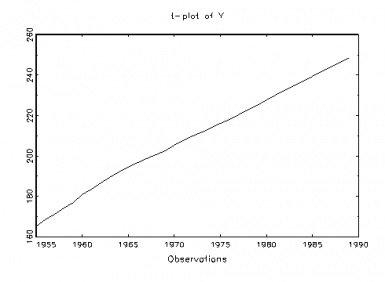
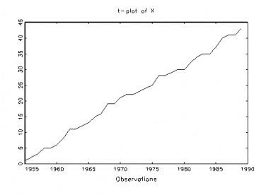
Here are two plots (t-plots) of the observed data where yt is the population of the USA in millions, and  xt our “secret” variable, to be revealed later on, both over time (1955-1989).

Fig 1: USA Population (y)

Fig 1: USA Population (y)

mstestingPart2Fig2

Fig. 2: Secret variable (x)

mstestingPart2 Fig 3

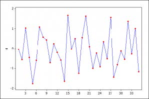
Figure 3: A typical realization of a NIID process.

Pretty clearly, there are glaring departures from IID when we compare a typical realization of a NIID process,  in fig. 3, with the t-plots of the two series  in figures 1-2.  In particular, both data series show the mean is increasing with time – that is, strong mean-heterogeneity (trending mean).Our recommended next step would be to continue exploring the probabilistic structure of the data in figures 1 and 2  with a view toward thoroughly assessing the validity of the LRM assumptions [1]-[5] (table 1). But first let us take a quick look at the traditional approach for testing assumptions, focusing just on assumption [4] traditionally viewed as error non-autocorrelation: E(ut,us)=0 for t≠s, t,s=1,2,…,n. Continue reading

Categories: Intro MS Testing, Statistics | Tags: , , , , ,

Intro to Misspecification Testing: Ordering From A Full Diagnostic Menu (part 1)


“This is the kind of cure that kills the patient!”

is the line of Aris Spanos that I most remember from when I first heard him talk about testing assumptions of, and respecifying, statistical models in 1999.  (The patient, of course, is the statistical model.) On finishing my book, EGEK 1996, I had been keen to fill its central gaps one of which was fleshing out a crucial piece of the error-statistical framework of learning from error: How to validate the assumptions of statistical models. But the whole problem turned out to be far more philosophically—not to mention technically—challenging than I imagined.I will try (in 3 short posts) to sketch a procedure that I think puts the entire process of model validation on a sound logical footing.  Thanks to attending several of Spanos’ seminars (and his patient tutorials, for which I am very grateful), I was eventually able to reflect philosophically on aspects of  his already well-worked out approach. (Synergies with the error statistical philosophy, of which this is a part,  warrant a separate discussion.)

Continue reading

Categories: Intro MS Testing, Statistics | Tags: , , , ,

RMM-4: Special Volume on Stat Scie Meets Phil Sci

The article “Foundational Issues in Statistical Modeling: Statistical Model Specification and Validation*” by Aris Spanos has now been published in our special volume of the on-line journal, Rationality, Markets, and Morals (Special Topic: Statistical Science and Philosophy of Science: Where Do/Should They Meet?”)

Abstract:
Statistical model specification and validation raise crucial foundational problems whose pertinent resolution holds the key to learning from data by securing the reliability of frequentist inference. The paper questions the judiciousness of several current practices, including the theory-driven approach, and the Akaike-type model selection procedures, arguing that they often lead to unreliable inferences. This is primarily due to the fact that goodness-of-fit/prediction measures and other substantive and pragmatic criteria are of questionable value when the estimated model is statistically misspecified. Foisting one’s favorite model on the data often yields estimated models which are both statistically and substantively misspecified, but one has no way to delineate between the two sources of error and apportion blame. The paper argues that the error statistical approach can address this Duhemian ambiguity by distinguishing between statistical and substantive premises and viewing empirical modeling in a piecemeal way with a view to delineate the various issues more effectively. It is also argued that Hendry’s general to specific procedures does a much better job in model selection than the theory-driven and the Akaike-type procedures primary because of its error statistical underpinnings.

Categories: Philosophy of Statistics, Statistics | Tags: , ,

Blog at WordPress.com.