

.
This is a modified reblog of an earlier post, since I keep seeing papers that confuse this.
Suppose you are reading about a result x that is just statistically significant at level α (i.e., P-value = α) in a one-sided test T+ of the mean of a Normal distribution with n iid samples, and (for simplicity) known σ: H0: µ ≤ 0 against H1: µ > 0.
I have heard some people say:
A. If the test’s power to detect alternative µ’ is very low, then the just statistically significant x is poor evidence of a discrepancy (from the null) corresponding to µ’. (i.e., there’s poor evidence that µ > µ’ ).*See point on language in notes.
They will generally also hold that if POW(µ’) is reasonably high (at least .5), then the inference to µ > µ’ is warranted, or at least not problematic.
I have heard other people say:
B. If the test’s power to detect alternative µ’ is very low, then the just statistically significant x is good evidence of a discrepancy (from the null) corresponding to µ’ (i.e., there’s good evidence that µ > µ’).
They will generally also hold that if POW(µ’) is reasonably high (at least .5), then the inference to µ > µ’ is unwarranted.
Which is correct, from the perspective of the (error statistical) philosophy, within which power and associated tests are defined?
(Note the qualification that would arise if you were only told the result was statistically significant at some level less than or equal to α rather than, as I intend, that it is just significant at level α, discussed in a comment due to Michael Lew here [0])
Allow the test assumptions are adequately met (though usually, this is what’s behind the problem). I have often said on this blog, and I repeat, the most misunderstood and abused (or unused) concept from frequentist statistics is that of a test’s power to reject the null hypothesis under the assumption alternative µ’ is true: POW(µ’). I deliberately write it in this correct manner because it is faulty to speak of the power of a test without specifying against what alternative it’s to be computed. It will also get you into trouble if you define power as in the first premise in a recent post:the probability of correctly rejecting the null
–which is both ambiguous and fails to specify the all important conjectured alternative. [For slides explaining power, please see this post.] That you compute power for several alternatives is not the slightest bit problematic; it’s precisely what you want to do in order to assess the test’s capability to detect discrepancies. If you knew the true parameter value, why would you be running an inquiry to make statistical inferences about it?
It must be kept in mind that inferences are going to be in the form of µ > µ’ =µ0 + δ, or µ < µ’ =µ0 + δ or the like. They are not to point values! (Not even to the point µ =M0.) Most simply, you may consider that the inference is in terms of the one-sided lower confidence bound (for various confidence levels)–the dual for test T+.
DEFINITION: POW(T+,µ’) = POW(Test T+ rejects H0;µ’) = Pr(M > M*; µ’), where M is the sample mean and M* is the cut-off for rejection at level α . (Since it’s continuous it doesn’t matter if we write > or ≥). I’ll leave off the T+ and write POW(µ’).
In terms of P-values: POW(µ’) = Pr(P < p*; µ’) where P < p* corresponds to rejecting the null hypothesis at the given level.
Let σ = 10, n = 100, so (σ/ √n) = 1. Test T+ rejects H0 at the .025 level if M > 1.96(1). For simplicity, let the cut-off, M*, be 2.
Test T+ rejects H0 at ~ .025 level if M > 2.
CASE 1: We need a µ’ such that POW(µ’) = low. The power against alternatives between the null and the cut-off M* will range from α to .5. Consider the power against the null:
1. POW(µ = 0) = α = .025.
Since the the probability of M > 2, under the assumption that µ = 0, is low, the just significant result indicates µ > 0. That is, since power against µ = 0 is low, the statistically significant result is a good indication that µ > 0.
Equivalently, 0 is the lower bound of a .975 confidence interval.
2. For a second example of low power that does not use the null: We get power of .04 if µ’ = M* – 1.75 (σ/ √n) unit –which in this case is (2 – 1.75) .25. That is, POW(.25) =.04.[ii]
Equivalently, µ >.25 is the lower confidence interval (CI) at level .96 (this is the CI that is dual to the test T+.)
CASE 2: We need a µ’ such that POW(µ’) = high. Using one of our power facts, POW(M* + 1(σ/ √n)) = .84.
3. That is, adding one (σ/ √n) unit to the cut-off M* takes us to an alternative against which the test has power = .84. So µ = 2 + 1 will work: POW(T+, µ = 3) = .84. See this post.
Should we say that the significant result is a good indication that µ > 3? No, there’s a high probability (.84) you’d have gotten a larger difference than you did, were µ > 3.
Pr(M > 2; µ = 3 ) = Pr(Z > -1) = .84. It would be terrible evidence for µ > 3!
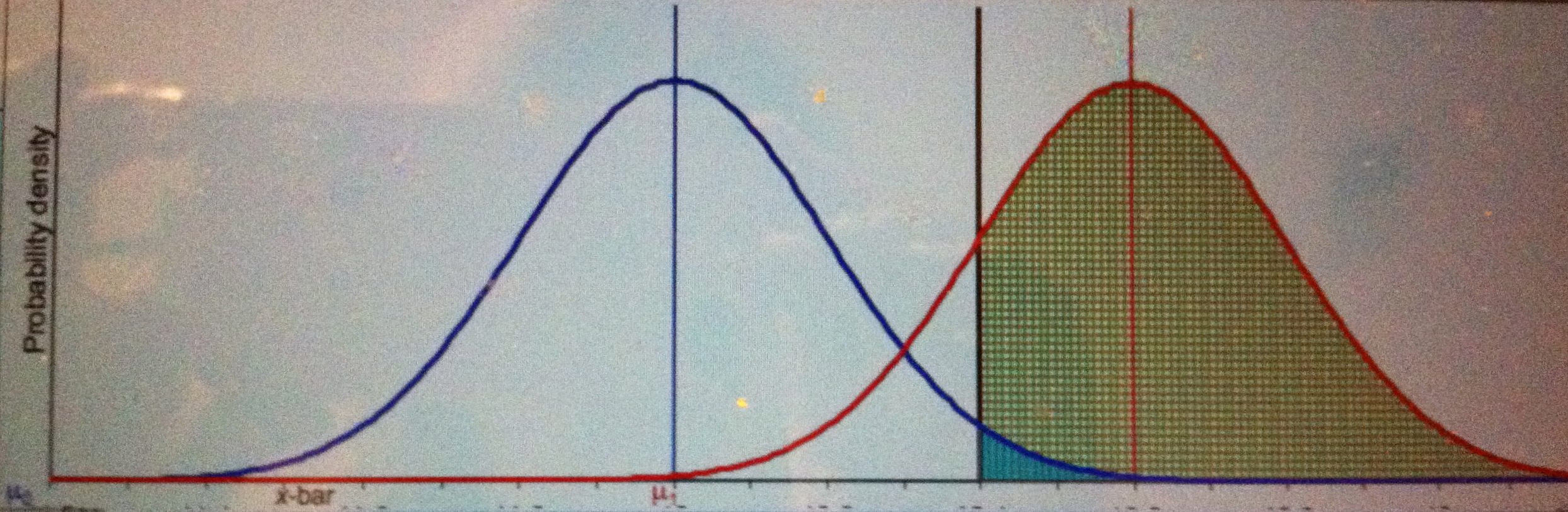
Blue curve is the null, red curve is one possible conjectured alternative: µ = 3. Green area is power, little turquoise area is α.
Note that the evidence our result affords µ > µ’ gets worse and worse as we pull µ further and further to the right, even though in so doing we’re increasing the power.
As Stephen Senn points out (in my favorite of his guest posts), the alternative against which we set high power is the discrepancy from the null that “we should not like to miss”, delta Δ. Δ is not the discrepancy we may infer from a significant result (in a test where POW(Δ) = .84).
So the correct answer is B.
Does A hold true if we happen to know (based on previous severe tests) that µ <µ’?
No, but it does allow some legitimate ways to mount complaints based on a significant result with low power to detect a known discrepancy.
(1) It does mean that if M* (the cut-off for a result just statistically significant at level α) is used as an estimate of µ and we know that µ < M*, then M* is larger than µ. So your observed result, which we’re assuming is M*, “exaggerates” µ, were you to use it as an estimate, rather than using the lower limit of a confidence bound. This is not power analysis.
(2) However, knowing the test had little capability of detecting the effect sizes deemed true, it might raise the question of whether the researchers cheated, and this, I claim, is a plausible reason to suspect the result. If the study is in a field known to have lots of researcher flexibility, and the power to detect discrepancies in the ballpark known independently to be correct is low, then you might rightly suspect that they cheated. They reported only the one impressive result after trying and trying again, or tampered with the discretionary points of the study to achieve nominal significance. This is a different issue, and doesn’t change my answer. More generally, it’s because the answer is B that the only way to raise the criticism legitimately is to challenge the assumptions of the test.
Why do people raise the criticism illegitimately? In some circles it’s a direct result of trying to do a Bayesian computation and setting about to compute Pr(µ = µ’|Mo = M*) using POW(µ’)/α as a kind of likelihood ratio in favor of µ’. I say this is unwarranted, even for a Bayesian’s goal, see 2/10/15 and 5/22/16 posts below. Notice that supposing the probability of a type I error goes down as power increases is at odds with the trade-off that we know holds between these error rates. So this immediately indicates a different use of terms.
*Point on language: “to detect alternative µ'” means, “produce a statistically significant result when µ = µ’.” It does not mean we infer µ’. Nor do we know the underlying µ’ after we see the data, obviously. Perhaps the strict definition should be employed unless one is clear on this. The power of the test to detect µ’ just refers to the probability the test would produce a result that rings the significance alarm, if the data were generated from a world or experiment where µ = µ’.
[0] Since power is what’s used in the articles we’re considering, rather than the data-dependent computation of severity, by making the result just significant at level α, we make the assessment equal.
[i] I surmise, without claiming a scientific data base, that this fallacy has been increasing over the past few years. It was discussed way back when in Morrison and Henkel (1970). (A relevant post relates to a Jackie Mason comedy routine.) Research was even conducted to figure out how psychologists could be so wrong. Nowadays it’s because of the confusion introduced by computing a “positive predictive value” and transposing the ‘conditional’.
[ii] Pr(M > 2; µ = .25 ) = Pr(Z > 1.75) = .04.
OTHER RELEVANT POSTS ON POWER
- (3/4/14) Power, power everywhere–(it) may not be what you think! [illustration]
- (3/12/14) Get empowered to detect power howlers
- 3/17/14 Stephen Senn: “Delta Force: To what Extent is clinical relevance relevant?”
- (3/19/14) Power taboos: Statue of Liberty, Senn, Neyman, Carnap, Severity
- 12/29/14 To raise the power of a test is to lower (not raise) the “hurdle” for rejecting the null (Ziliac and McCloskey 3 years on)
- 01/03/15 No headache power (for Deirdre)
- 02/10/15 What’s wrong with taking (1 – β)/α, as a likelihood ratio comparing H0 and H1?
- 5/22/16 Frequentstein:What’s wrong with taking (1 – β)/α, as a measure of evidence against the null?


")


I thought of an analogy that might help. Imagine you are performing on American Idol or another one of these singing shows. You know there are two judges: the first is extremely critical and has a high probability of bringing up even small flaws in your performance (the “high-powered” test) and another who is easier, and only has a high probability of bringing up big flaws (the “low-powered” test). When do we learn the most from each judge?
From the critical judge, we learn the most when they don’t bring up any flaws, and we can then infer that it was a good performance (small discrepancy from an “ideal” performance). This is analogous to a nonsignificant result from a high-powered test.
From the uncritical judge, we learn the most when they *do* bring up flaws. If that judge says they dislike our performance, then we can infer that it was pretty bad (large discrepancy from an “ideal” performance). This is analogous to a significant result from a low-powered test.
We learn very little when the critical judge scowls at us because they almost always will hate something. Likewise, we learn very little when the uncritical judge fails to bring up anything because they are so easy-going.
Finally, knowing that the critical judge would definitely scowl at us if we gave a very bad performance does not mean that we can take his scowl to mean that we actually gave an awful performance. If we thought that way, we would never be happy with our performance! (That is, we would almost always infer that our performance was very different from ideal, even when it wasn’t). The scowl from the critical judge could mean that we gave a very good performance (close to ideal), but he’s just very critical. This is analogous to the situation with power: we cannot take rejection by a high-powered test to mean that there is a large effect.
Richard: Thanks, I often use my smoke alarm analogy: when you hear the alarm that doesn’t go off unless your whole house is ablaze it’s more of an indication of fire than when you hear the one that goes off with burnt toast. You need a measurement that can be more or less extreme, e.g, growing amount of fire. But I guess we can imagine a measure of goodness of performance, in your example. The part that should be most obvious is your point:
“Finally, knowing that the critical judge would definitely scowl at us if we gave a very bad performance does not mean that we can take his scowl to mean that we actually gave an awful performance.”
Right:
Bad performance => scowl.
scowl.
—–
bad performance
is (the invalid) affirming the consequent, here of the statistical sort. It’s a logic affirmed by Bayes Theorem, in the sense that a B-boost confirms. That’s why they [Bayesians, some of them) say they “solve” the problem of induction, because the logic of
H => e
e
—-
H
is endorsed. Severe testers wouldn’t want to endorse such an induction since it’s unreliable (w/o adding the severity requirement) but it’s at the heart of things.
Interpretation B is also appropriate for an “objective Bayesian” using a vague/uniform/uninformative prior ( which I am not advocating).
Case 1: Posterior Probability ( µ > µ’ | x=M*) = 0.96
Case 2: Posterior Probability ( µ > µ’ | x=M*) = 0.16
Which has a direct interpretation in contrast to the power approach “… there’s a high probability (.84) you’d have gotten a larger difference than you did”
Andy: Sure, I wasn’t claiming all Bayesian positions get this wrong, certainly matching ones would match. But, as I see it, it’s “the power approach” (using your language) that gives the direct basis for assessing well-testedness (of claims about the origins of the data). I never know what something like Pr( µ > µ’ | x=M*) = 0.16 means? Is it low -ish belief in µ > µ’ ? or µ > µ’ occurs with prob .16 given x =M*. Anyway, that’s a different issue.
I never know what something like Pr( µ > µ’ | x=M*) = 0.16 means. Is it low -ish belief in µ > µ’ ? or µ > µ’ occurs with prob .16 given x =M*
I am surprised at this comment, so here’s an answer.
Using the probability calculus to describe what is known, µ isn’t stochastic so it can’t be the latter. It’s the former; conditional on the observed data x=M*, and all relevant modeling assumptions including whatever the prior was, 0.16 of the posterior knowledge lies above µ’.
One might not agree with the premise that what’s known should be described in terms of probability calculus – but if one does accept it, getting to basic Bayesian inferences such as this is essentially automatic.
George: So, Pr( µ > µ’ | x=M*) = 0.16 would mean, µ isn’t stochastic, but what I know about it is .16? This is very thin, murky. I’m not pretending I can’t imagine ways to cash it out, the best of which seems to be something like: I’d bet on µ > µ’ in the way I’d bet on an event with known probability .16. Is that what you mean?
My position is, basically, let’s grant this betting meaning. I don’t think the error probability quantities (that we were talking about) translate into betting probabilities, nor that betting reports are the direct aim of using statistics in science. I distinguish such an aim from the task of using statistics to quantify how well or severely tested a claim is. I might strongly believe a claim C, but deny that data x from test T has probed C well at all. C can be plausible, but horribly tested by x. One needn’t deny the probabilist goal in order to recognize this distinct goal. I see error probabilities as characterizing the capacity of a method to have probed ways in which C may be false. Even if the data x accord with C, it’s not warranted with severity if such good or even better accordance is fairly easy to achieve (frequent) even if C is specifiably false.The growth of knowledge isn’t in terms of updating beliefs but rather the growth of information, theories, models, and capabilities to solve problems and learn more. All this will sound very Popperian and it is, but Popper was never able to fully explicate his insights. You might see my slides from my previous post (a commentary on Nancy Reid).
You might see my slides from my previous post (a commentary on Nancy Reid).
Thanks, I already read these, with interest.
So, Pr( µ > µ’ | x=M*) = 0.16 would mean, µ isn’t stochastic
In the mode of thought I’m considering, µ is never stochastic. Probability is just a set of rules – a grammar, if you like – for describing what’s known about fixed parameters. If the arguments for it being a sensible grammar don’t convince, pragmatists will note it happens to be a grammar that makes it very easy to update knowledge in the light of data that wasn’t previously used.
Specifically for this example, Pr( µ > µ’ | x=M*) = 0.16 is a summary of the posterior knowledge for µ, saying that given data x=M* (and some implicit modeling steps, including a prior) 0.16 of the support for µ lies above µ’. That’s all.
My position is, basically, let’s grant this betting meaning.
One need not invoke betting to use this language, so there’s little to say here.
The growth of knowledge isn’t in terms of updating beliefs but rather the growth of information, theories, models, and capabilities to solve problems and learn more.
Regarding well-testedness – which I do think is interesting – it would really help to have examples where this differs importantly from reasonable interpretations of sensibly-constructed confidence (or credible) intervals, which give an indication of how different the truth would have to be in order to give a different testing outcome. I have tried to find such examples but without success, and would be grateful to anyone who can point me to them.
Finally, pursuing a goal which is as open-ended as you suggest (“the growth of information, theories, models, and capabilities to solve problems and learn more”) sounds very distant from the approach of most theoretical work in statistics. There, even fairly specific measures of optimality (e.g. efficiency of estimates) are hard-won – see e.g. Le Cam’s work. It therefore seems unlikely that one could show that a particular way of proceeding provides all your goals; even just defining them rigorously enough to start assessing properties seems a challenge.
George: There’s too much I could say to your interesting comment. Some initial thoughts.
“Probability is just a set of rules – a grammar, if you like – for describing what’s known about fixed parameters. If the arguments for it being a sensible grammar don’t convince, pragmatists will note it happens to be a grammar that makes it very easy to update knowledge in the light of data that wasn’t previously used.”
I don’t understand how these probabilities describe what is known, and if they fail to represent what’s known, it’s not obviously relevant pragmatically to state that they make it easy to update what’s known. Even alluding to an uncontroversial case of the probability of an event (not a statistical hypothesis), it needs to be cashed out. Generally it’s in terms of how frequently the event would occur in some hypothetical population. How does this work in describing “what is known” about parameters? I’m not sure how describing it as a “grammar” helps to make the numbers relevant for empirical inquiry.
“Regarding well-testedness – which I do think is interesting – it would really help to have examples where this differs importantly from reasonable interpretations of sensibly-constructed confidence (or credible) intervals, which give an indication of how different the truth would have to be in order to give a different testing outcome.”
Since this is to provide an inferential interpretation and rationale of existing (error statistical) methods like CIs, it wouldn’t make sense for an intuitively plausible assessment of well-testedness to be at odds numerically with a good or best CI–even if there are differences in interpretation. It’s what’s poorly tested that will differ. For ex. points within a CI are non-rejectable at a given level, but they may be very poorly tested.
If there was no controversy surrounding the right interpretation and justification of existing methods, there would perhaps be no need for recognizing a different goal, but that’s not the case. If it turns out to underlie the implicit aim of existing methods, lying below the stated goals–that’s all to the good, that’s my hope. But I’ve never seen it defended or used to adjudicate current criticisms.
“It therefore seems unlikely that one could show that a particular way of proceeding provides all your goals”.
This is a piecemeal approach; I didn’t say a single application of a stat procedure would do all this, I was just trying to suggest a view that stands as a rival to an aim that is thought to be uncontroversial but which isn’t argued for e.g.,formal degrees of belief, and updating them. (The “growth of knowledge” goes beyond formal statistical aims.) Explaining what’s wrong with inferring poorly tested claims, and why we’d want claims that survive stringent testing isn’t at all difficult. What’s the reason for desiring a grammar to assign numbers, when I don’t know what they mean or how to use them or why it’s thought one particular choice of grammar expresses knowledge?
Thanks for the replies, particularly on “implicit aims”. Am also trying to avoid writing too much, so please excuse the partial response:
I don’t understand how these probabilities describe what is known.
I think you’re up against an axiom there; it’s a baked-in part of the Bayesian approach that information can be encoded in this way, i.e. that there is some fixed total amount of knowledge that it’s spread out over possible (but unknown) true states of Nature, and that the support for the union of disjoint sets of states of Nature is the sum of their supports.
With regard to “cashing out” (which I interpret as just considering the consequences of these axioms) it’s fairly obvious that this grammar means one cannot end up supporting states of Nature one did not support a priori, which seems like a weakness. But it is possible to end up with Bayesian inferences along the lines of “here’s what we now believe about Nature, and also that the data we observed is nevertheless nothing like what we’d expect under those states of Nature”. So this weakness is perhaps not so bad as it first seems; at least in a practical sense models can still be checked against data, and perhaps rejected.
Other consequences of the axioms are, well, all of probability theory. Despite their simplicity the axioms are known for providing an immensely rich grammar: therefore it’s reasonable to require those who maintain Bayes can’t provide the inferences they seek to strongly justify their claims.
Foregoing the probability grammar to describe knowledge, one can either have no grammar at all, or some alternative. With no grammar, there seems (to me) to be no principles against which to evaluate difference procedures. i.e. no way of saying whether inferences are appropriate or not. With some other non-Bayesian grammar it is extremely difficult to rule out incoherence, which seems a serious shortcoming for a scientific system.
George: Thanks for your comment.
You say “I think you’re up against an axiom there; it’s a baked-in part of the Bayesian approach..”.
No empirical claim “comes up against an axiom”, because an axiom is a mere piece of syntax that only gets its meaning, and thus the possibility of being true and open to appraisal, by giving it a semantics. The creator of a formal system sets out axioms by fiat, and the grammar is also a piece of syntax. The Bayesian meaning, you say, “baked in” to the approach is degree of knowledge or how much “information”. What needs to be substantiated is that any resulting assertions, now being given meanings, latch up with what is taken to be true about information, inference, knowledge. A more common semantics is in terms of betting, and people argue as to whether the resulting claims holds true for bets, but you have nixed that (I’m not saying that’s had great success). So you’d have to show why your semantics is adequate for expressing truths about knowledge and inference, or whatever you have in mind. Few people, these days, think probability logic captures how people actually make inferences, but it might be alleged, as it often is, that they ought to reason this way if they were rational, or the like. Is that what you’d aver in the case of your semantics?
No one is ever robbed of using a formal system or logic, and (having started life as a formal logician) I’m aware of quite a few logics out there that could be contenders for representing epistemic stances—given the right semantics. Logics can be assured to be deductively valid (so long as they’re created consistently) but that means very little when it comes to soundness. The trick is to show that what’s derivable from your axioms captures what’s true about the domain of interest–and conversely.
Thank you for this informative posts! Also enjoyed the analogy that Richard added in the comments. It does make some intuitive sense that if power against a particular alternative is low, then a (barely) significant results is good evidence of a discrepancy, because under low power, we need to observe a pretty big difference between mu and mu’. Otherwise, it wouldn’t be significant.
I am reminded of this quote by James Heckman where he said (in the context of some early intervention program):
“The fact that samples are small works against finding any effects for the programs, much less the statistically significant and substantial effects that have been found.”
It seems to be that he is employing reasoning of the type B that you outlined in your post.
But I do wonder why Andrew Gelman refers to this as the “What does not kill my statistical significance makes it stronger” fallacy. (http://andrewgelman.com/2017/02/06/not-kill-statistical-significance-makes-stronger-fallacy/). He seems concerned that under a low power situation, a sig. effect will likely be very much exaggerated – what he calls the Type M error. I know that you are very familiar with Gelman’s work, but I would love to hear your comment on that. And maybe there is no contradiction here – it could be good evidence against a hypothesis, and at the same time an exaggerated point estimate of the alternative.
In trying to fit this into Richard’s analogy… if the true (unobserved) flaw of the singer is small, then a detection of the low-powered, uncritical judge, meaning the judge points out a flaw, means that we have good evidence that this is not a perfect performance, but at the same time, the magnitude of the flaw is highly exaggerated, because otherwise the uncritical judge would not have mentioned this flaw.
What does this then imply for researchers who are operating in such a situation – take for example Heckman’s research. Are we supposed to believe that the effect of the early-childhood intervention is likely real, but the effect likely over-estimated?
And just to be clear, I am not bringing up Gelman’s post and asking this to stoke an argument – I am genuinely interested in understanding some of the involved nuances.
Thanks!
Felix:
I don’t think I’ve quite convinced you of my point, at least when you write: “if power against a particular alternative is low, then a (barely) significant results is good evidence of a discrepancy, because under low power, we need to observe a pretty big difference between mu and mu’.” It’s not really wrong, but makes it sound exceptional.
Every test will have low power to detect discrepancies close enough to Ho, because the power at Ho is alpha. In the test I described, T+, the power goes from alpha to .5 when we consider discrepancies ranging from o to the cut-off (which I wrote here as M*). The power only grows greater than .5 for alternatives larger than the cut-off M*. So there’s not something unkosher or unusual about making inferences about the mu values between the null and M*. On the contrary, that’s what tests always do. It’s because getting an M > M* is improbable under the null that we take M* as indicating the true mu exceeds 0 (the null value). Values of mu just slightly greater than 0 work the same way although our evidence that mu exceeds them isn’t as strong as that mu exceeds 0. Of course all of these inferences imply mu > 0, so logic alone tells us their warrant is less than that for mu > 0. Once again, it’s the improbability of getting M > M* under mu = mu’ (i.e., POW(mu’) = low) that underwrites taking M* as an indication that the data were generated from a world where mu > mu’.
As for Gelman and Carlin, take a look at what I say in the section that asks whether the answer to my question is any different if we knew the true mu was a value mu’ that the test had little power against. The answer doesn’t change, but clearly M* exceeds mu’, so if you knew mu = mu’, you’d know M* exceeds the true mu. So if you used M* to estimate mu–rather than the lower confidence bound–, then your estimate would exceed the true mu value. I think the strongest point is that one might very well suspect cheating, biased selection effects and the like, if M* is observed and is so clearly out of whack that even the lower confidence bound is out of whack with what’s known from background. That’s the only way I can make sense of their position. So, as you say, there may be no contradiction.
I don’t really know their work well, so if someone has a different explanation of their point I’d be glad to hear it. I inquired at one stage, and I don’t think we settled it.
Mayo:
Your reply is much appreciated. It’s possible that I didn’t fully get your point. I interpreted your two cases at the beginning of your blog as a situation in which mu’ is the same for both tests, and the sample size differs. So, scenario A has small n and low power for mu’, and scenario B has high n, high power for (the same) mu’. Both have identical p-values of .05 (just statistically significant result). In that case, scenario A would have to observe a larger deviation in the sample, as in Richard’s analogy of critical and uncritical judges.
To flesh this out a bit. Consider one case in which n=10, sd=1, and true mu in population is .1. For this to yield p=.05, I would need to see a deviation of roughly .62 (assumming here a critical cut-off of t=2). For n=1000, sd=1, and true mu in pop of .1, I need a deviation of .062 to yield p=.05. Power of these two tests for mu=0 against mu1=.1 is around 10% and over 90%, respectively. To me this mapped on to Richard’s analogy of the uncritial and critical judge. The n=10, low-powered test, hits only if deviation from 0 is quite large. The n=1000, high-powered test, hits if deviation from 0 is quite small. If they both have exactly p=.05, then in low-powered scenario I necessarily must have observed a larger deviation. Hopefully, this goes in the right direction of what you intended to convey.
I did notice that in your later examples where you flesh the scenarios out in the middle part, you consider a situation in which n is fixed throughout, and mu’ changes across scenarios, so maybe I am missing an additional point that you tried to make.
Felix: What you say is right, but “big” is relative. Also, if the sample size is too small, affirming the assumptions hold even reasonably adequately is threatened.
Thank you Mayo – I enjoyed this blog post and the small discussion. It made me think more deeply about statistical power, and hopefully I can integrate some of these thoughts in my teaching.