

.
Stephen Senn
Consultant Statistician
Edinburgh, Scotland
The Many Halls Problem
It’s not that paradox but another
Generalisation is passing…from the consideration of a restricted set to that of a more comprehensive set containing the restricted one…Generalization may be useful in the solution of problems. George Pólya [1] (P108)
Introduction
In a previous blog https://www.linkedin.com/pulse/cause-concern-stephen-senn/ I considered Lord’s Paradox[2], applying John Nelder’s calculus of experiments[3, 4]. Lord’s paradox involves two different analyses of the effect of two different diets, one for each of two different student halls, on weight of students. One statistician compares the so-called change scores or gain scores (final weight minus initial weight) and the other compares final weights, adjusting for initial weights using analysis of covariance. Since the mean initial weights vary between halls, the two analyses will come to different conclusions unless the slope of final on initial weights just happens to be one (in practice, it would usually be less). The fact that two apparently reasonable analyses would lead to different conclusions constitutes the paradox. I chose the version of the paradox outlined by Wainer and Brown [5] and also discussed in The Book of Why[6]. I illustrated this by considering two different experiments: one in which, as in the original example, the diet varies between halls and a further example in which it varies within halls. I simulated some data which are available in the appendix to that blog but which can also be downloaded from here http://www.senns.uk/Lords_Paradox_Simulated.xls so that any reader who wishes to try their hand at analysis can have a go.
I showed that Nelder’s calculus reveals that there is no solution if the diet is varied between halls. This is because replication is needed at the level at which treatment is varied and two halls, one per treatment provides insufficient replication. In this blog I shall present a simulated example that provides more replication at the level of hall. In order to keep numbers manageable in the previous example I simulated data for 40 students in total, 20 per hall. In the new example, in order to underline the point that it is not the total number of students that is the problem, I shall stick to 40 students but will have them in ten halls, so four per hall. Of course, in practice this would be a ludicrously low number of students for any hall but that is irrelevant to the understanding of the problem. However, if one wishes to make the example seem more practical, assume that resources to carry out measurements are limited and to make the study feasible, four students from each hall have been chosen at random to be followed.
I shall present the simulated data in due course but first let me dispose of some red herrings.
Tedious objections
A tedious objection that has been raised to the example previously presented is that an observational study was originally proposed by Lord and I have offered an experiment, which is irrelevant. This objection is just silly on several grounds. The first point to note is that Lord’s paradox is not dependent on an observational study having been conducted. The paradox is a numerical phenomenon. It will still arise if an experiment in conducted. Furthermore, the fact that an experiment has been conducted gets rid of many possible distracting factors revealing the paradox in a purer form. The second point is that whereas one can imagine analyses that would succeed in an experiment but fail in an observational study, the reverse is not the case. Therefore, since I showed that the proposed solution to the paradox would be problematic if an experiment had been carried out the objection cannot be avoided by switching to an observational study. The third point is that it is surely a fatal weakness of any causal theory that it has nothing to say about experiments. I think highly enough of the theory outlines in The Book of Why to conclude that it does not suffer from this defect, so it is reasonable to measure it against experiments.
A second tedious objection is that by considering a case with many halls I am not looking at Lord’s Paradox. My reply to this is to say that two is a special case (albeit a restricted one) of many. Sometimes to understand problems properly one has to generalise and, indeed, sometimes generalisation can make a solution easier. (See Pólya’s advice in the opening quotation.)
The example
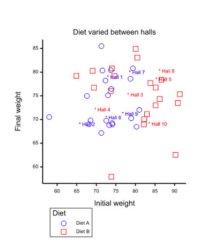
Figure 1 Scatter plot of final against initial weights for 40 students. Five halls have used diet A (blue circle) and five have used diet B (red square). Hall means are indicated by asterisks.
I am going to consider a many halls problem (not be confused with the famous Monty Hall problem). I simulated data for ten halls, five each being allocated diet A and five being allocated diet B. In each hall four students were followed and their initial weights at the start of the academic year and their final weights, at the end were measured. Other parameters of the simulation are given in my previous blog https://www.linkedin.com/pulse/cause-concern-stephen-senn/, however, unlike in the previous blog I avoid the complication of a second level of experimentation in which dietary advice is varied within halls. The 40 pairs of measurements are represented by the scatter plot in Figure 1 and are given in the appendix.
Blue circles represent values for student’s allocated to halls that used diet A and red squares values for students in halls that used diet B. The mean values per hall are represented by asterisks and the colour blue is used for diet A and red for diet B.
I can now analyse the values using John Nelder’s calculus of experiments as implemented in Genstat® as follows
BLOCKSTRUCTURE Hall/Student
COVARIATE X
The first statement informs the algorithm that the ‘experimental material’ consists of students within halls. The second declares the initial weight X (labelled Initial in output) as a covariate. If the following statement is added
TREATMENTSTRUCTURE Between
the algorithm is informed of the treatment factor of interest, which I have called Between because it is varied between halls (the output labels it as diet). If I now instruct it to carry out an analysis of variance on the outcome variable , Y (labelled Final, in output) , as follows
ANOVA[FPROBABILITY = YES] Y
the instructions are complete. The output is given in Figure 2. The following points are important. First, the significance of the effect of treatment is judged by using the variation between halls. The output distinguishes two strata: the Hall stratum and the Hall.Student stratum. Only the former is used in judging the effect of treatment because the treatment has been varied between halls. It would be a mistake, analogous to analysing a cluster randomised trial[7] as if it were a parallel group trial, to use the Hall.Student stratum to judge the effect of diet. The second point is that there are different regression coefficients between and within halls. The former is estimated to be 0.42 ( I had set it to 0.5 for the simulation) and the latter to 0.957 (I had set it to 0.8 for the simulation). Given the level at which treatment is varied, the first of these and not the second is relevant for adjusting final weights. See Yoon and Welsh for a general investigation of correlations for multilevel data[8] and Kenward and Roger for the issue as it occurs in cross-over trials[9]. For earlier discussions of technical matters to do with more complex multi-level experiments see Zelen [10], Ratcliff et al [11] and Payne and Tobias[12].
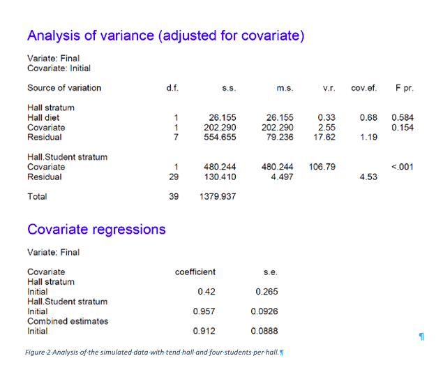
Figure 2 Analysis of the simulated data with tend hall and four students per hall.
Lessons for the two-hall problem
There are two obvious lessons for the two-hall problem. The first is that variation has to be judged at the hall level not the within-hall level. A consequence of this is that since there are only two halls, there are not enough degrees of freedom to do this whether or not a simple change-score analysis or analysis of covariance is used. The second is that covariation also has to be judged at the between-hall level and again this cannot be estimated. A consequence of the second point is that it is no defence of a proposed solution based on using the within-halls regression coefficient to say that one is not interested in standard errors but only in the asymptotic solution. The estimate itself is wrong, unless it can be assumed that the between-hall regression will be the same as the within-hall one[13]. The latter coefficient is estimate as 0.96 but the former at 0.42.
Note that had the design been that students from across the university had been allocated at random to one of two diets, then the conventional ANCOVA solution which, as far as I can tell, is the one proposed in The Book of Why[6] would have been correct. Furthermore, if students had been allocated to one of two diets based on initial weight (with those weighing less being allocated to one diet and those weighing more to another), then as Holland and Rubin have discussed[14], provided the regression may be assumed to be constant across the range of initial weight, the conventional ANCOVA solution works.
Can the ANCOVA solution be rescued?
Before discussing this, I want to make it quite clear that the change-score solution is a non-starter. It would rely on the assumption that the regression between halls was one and, in any case, estimation of the standard errors would be incorrect.
To rescue the ANCOVA solution, one device would be to move the Hall effect from the block structure to the treatment structure. One might also require some further assumptions. For example I could consider a case where students have been randomised to halls or perhaps allocated based on their weight, as discussed by Holland and Rubin[14] or I could just assume that given initial weight everything else is ignorable. Other assumptions regarding independence might be needed. If I do this and make Hall a fixed effect then Genstat® will tell me that Hall is confounded with Diet, however many halls I have, provided that the diet is varied between and not within halls.
Let us consider the two-hall case discussed in the previous blog. In the example I simulated, Hall 1 used diet B and Hall 2 used diet A. I might claim that I do not care what caused an effect on weight provided that I can identify there is some causal difference between the two groups. It may be diet B compared to A, it may be Hall 1 compared to 2 or it may be the combination of Hall 1 and diet B compared to Hall 2 and diet A.
This seems to me to be rather unambitious and does not get us very far in answering the Why that causal analysis is all about: it could be one thing it could be another or it could be both. At the very least it seems worth a discussion for anybody claiming that the ANCOVA solution is definitely correct.
In conclusion
I conclude by making one point regarding conditioning on effects. When you have hierarchical data-sets you can have variances and covariances at different levels and you can have more than one regression. For an analogy, think of stars moving relative to the centre of galaxies and galaxies being pulled by The Great Attractor. To say that you have conditioned on X under such circumstances is ambiguous. How have you conditioned? Or, to put it another way “How” have you answered “Why”?
As I have put it before, the consequence is that not only is correlation not necessarily causation, it may not even be correlation.
References
- Polya, G., How to solve it: A new aspect of mathematical method. 2004: Princeton university press.
- Lord, F.M., A paradox in the interpretation of group comparisons. Psychological Bulletin, 1967. 66: p. 304-305.
- Nelder, J.A., The analysis of randomised experiments with orthogonal block structure I. Block structure and the null analysis of variance. Proceedings of the Royal Society of London. Series A, 1965. 283: p. 147-162.
- Nelder, J.A., The analysis of randomised experiments with orthogonal block structure II. Treatment structure and the general analysis of variance. Proceedings of the Royal Society of London. Series A, 1965. 283: p. 163-178.
- Wainer, H. and L.M. Brown, Two statistical paradoxes in the interpretation of group differences: Illustrated with medical school admission and licensing data. American Statistician, 2004. 58(2): p. 117-123.
- Pearl, J. and D. Mackenzie, The Book of Why. 2018: Basic Books.
- Campbell, M.J. and S.J. Walters, How to Design, Analyse and Report Cluster Randomised Trials in Medicine and Health Related Research. Statistics in Practice, ed. S. Senn. 2014, Chichester: Wiley. 247.
- Yoon, H.-J. and A.H. Welsh, On the effect of ignoring correlation in the covariates when fitting linear mixed models. Journal of Statistical Planning and Inference, 2020. 204: p. 18-34.
- Kenward, M.G. and J.H. Roger, The use of baseline covariates in crossover studies. Biostatistics, 2010. 11(1): p. 1-17.
- Zelen, M., The analysis of incomplete block designs. Journal of the American Statistical Association, 1957. 52(278): p. 204-217.
- Ratcliff, D., E. Williams, and T. Speed, A note on the analysis of covariance in balanced incomplete block designs. Australian Journal of Statistics, 1984. 26(3): p. 337-341.
- Payne, R. and R. Tobias, General balance, combination of information and the analysis of covariance. Scandinavian Journal of Statistics, 1992: p. 3-23.
- Senn, S.J., Change from baseline and analysis of covariance revisited. Statistics in Medicine, 2006. 25(24): p. 4334–4344.
- Holland, P.W. and D.B. Rubin, On Lord’s Paradox, in Principals of Modern Psychological Measurement, H. Wainer and S. Messick, Editors. 1983, Lawrence Erlbaum Associates: Hillsdale, NJ. p. 3-25.
Appendix The Simulated Data
| Hall! | Student! | Between! | X | Y |
| 1 | 4 | A | 71.3 | 76.7 |
| 1 | 1 | A | 74.0 | 80.3 |
| 1 | 3 | A | 72.5 | 79.2 |
| 1 | 2 | A | 73.0 | 79.2 |
| 2 | 1 | A | 67.6 | 68.9 |
| 2 | 4 | A | 68.1 | 73.0 |
| 2 | 2 | A | 68.5 | 71.1 |
| 2 | 3 | A | 58.0 | 62.5 |
| 3 | 4 | B | 73.7 | 70.3 |
| 3 | 3 | B | 80.1 | 80.4 |
| 3 | 2 | B | 74.0 | 69.0 |
| 3 | 1 | B | 83.8 | 80.8 |
| 4 | 1 | B | 69.4 | 68.8 |
| 4 | 3 | B | 69.1 | 72.0 |
| 4 | 4 | B | 74.6 | 78.6 |
| 4 | 2 | B | 64.9 | 68.5 |
| 5 | 1 | B | 82.1 | 76.8 |
| 5 | 2 | B | 85.1 | 78.4 |
| 5 | 3 | B | 83.0 | 75.3 |
| 5 | 4 | B | 90.2 | 83.1 |
| 6 | 4 | A | 71.6 | 67.2 |
| 6 | 1 | A | 72.4 | 69.2 |
| 6 | 3 | A | 71.3 | 69.8 |
| 6 | 2 | A | 73.9 | 75.1 |
| 7 | 1 | A | 73.3 | 76.0 |
| 7 | 2 | A | 81.0 | 84.9 |
| 7 | 4 | A | 78.7 | 80.8 |
| 7 | 3 | A | 80.3 | 77.7 |
| 8 | 2 | B | 85.2 | 80.3 |
| 8 | 1 | B | 86.6 | 78.2 |
| 8 | 4 | B | 91.3 | 85.5 |
| 8 | 3 | B | 80.5 | 76.5 |
| 9 | 4 | A | 78.9 | 75.0 |
| 9 | 1 | A | 73.7 | 69.0 |
| 9 | 2 | A | 74.1 | 69.8 |
| 9 | 3 | A | 79.4 | 70.5 |
| 10 | 2 | B | 73.8 | 57.9 |
| 10 | 3 | B | 82.3 | 70.1 |
| 10 | 1 | B | 86.2 | 74.3 |
| 10 | 4 | B | 90.8 | 73.5 |
Simulated values. X stands for initial weight and Y for final weight.
The data are available at here http://www.senns.uk/Lords_Paradox_Ten_Halls.xls
Related guest post of Senn’s on this blog: Rothamsted statistics meets Lord’s paradox (Guest Post)


")


Dear Stephen:
Thank you so much for this intriguing guest post. I wonder if Pearl will respond in the comments as he did to a related post of yours in 2018:
Among his remarks:
“Thus, if the second statistician is not unambiguously right.
the first statistician cannot be unambiguously wrong.
If we exclude “untested assumptions” then no statistician
can be unambiguously right or unambiguously wrong.” (Pearl)
But this isn’t true in general. Your post is on a topic far removed from my expertise, but I thought your point was that John’s inference has a mistaken assumption whereas ambiguity remains with Jane’s analysis because there are different kinds of causal claims one might be asking about. (Or is that wrong?) As you say in your post:
How have you conditioned? Or, to put it another way “How” have you answered “Why”?
Given how equivocal are our “why” questions–especially when they are to be answered at the statistical, and not the individual, level–it seems a causal analysis should retain (and not claim to eliminate) ambiguity. Neither of the two attempts might give the “right” answer. Anyway, it’s interesting that (I think) you say Pearl’s analysis is in sync with randomly assigning all students to the two diets.
Pearl continues: “On the
other hand, if we accept “untested assumptions” they can tell us
unambiguously which statistician is right and which is wrong.
In either case, one of Senn’s conclusions must be wrong.” (Pearl)
But I thought the point of the ambiguity charge is that there are different “untested assumptions” one might assume.
Thanks, Deborah. The way I see it, Professor Pearl and I agree that one should condition on the initial weight and that this implies some sort of regression adjustment. We disagree because he assumes (I think) that this means the problem is solved whereas I don’t because the nature of the data means that there are different possible solutions to regressing on initial weight. This is the “how” problem I describe in this post. These are two questions I need to answer to know “how”.
1) How should we make this regression adjustment? (Correlation can occur at two levels so that there are at least two choices.)
2) How should we calculate a standard error for the effect of diet?
Standard ANCOVA would not, given the nature of the data-set, provide an answer to either of these questions without the following assumptions 1) the between-hall regression may be estimated using the within-hall regression 2) the final weights of students may be regarded as being conditionally independent given what else is in the model (diet and initial weight).
I think that these assumptions ought to be explicit and this is exactly what John Nelder’s (and Genstat’s) formal approach to the problem does. It renders them explicit.
I am no expert on DAGs but what I think is missing from the DAG is a term for “Hall”. As I describe in the post, one can excuse this by saying that Hall and Diet are the same thing. This, however, has implications for what one wishes to then conclude. For example, if there are several halls in the university and one wishes to use (say) diet B in all the halls because diet B in hall 2 proved better than diet A in hall 1 this will represent quite a challenge for any ‘fusion analysis’ (1) to follow.
For reasons, I have given elsewhere https://errorstatistics.com/2020/01/20/s-senn-error-point-the-importance-of-knowing-how-much-you-dont-know-guest-post/ I think that assessing uncertainty is central. So I think calculating ths standard errors correctly is a fundamental task. I would go further than this and suggest that concentrating on point estimates with the associated concept of unbiasedness has led to much confused thinking aboot “confounders”.
Reference
1. Bareinboim E, Pearl J. Causal inference and the data-fusion problem. Proceedings of the National Academy of Sciences. 2016;113(27):7345-7352. doi:10.1073/pnas.1510507113
Pingback: S. Senn: The Many Halls Problem (Guest Post) – 3ºB EE AMÁLIA RIBEIRO GARCIA PATTO – FILOSOFIA
Pingback: S. Senn: The Many Halls Problem (Guest Post) – 1ºs. C EE JOSÉ AYRTON FALCÃO- Sociologia
I love Lord Paradox (LP), as should every statistician, because it demonstrates so vividly, even more so than Simpson’s Paradox the need to abandon statistical orthodoxy and resort to causal analysis for its resolution. See https://ucla.in/2JeJs1Q and https://ucla.in/2YZjVFL
Senn’s recent posts on LP add a new color to its beauty: Even the heavy machinery of experimental design (which should, ostensibly, be adequate to deal with causal questions) remains helpless in resolving the paradox, for it lacks the vocabulary for articulating causal assumptions, nor the logic of moving from such assumptions to causal conclusions. Going through Senn’s posts, for example, I could not find a mathematical expression for the quantity we wish estimated, or for the assumptions one is willing to make to facilitate the estimation.
Where lies the problem?
Lord Paradox was originally posed as a phenomena observed in an observational study; students choose a dining hall (= diet) on their own volition and their final weight is determined (stochastically) by their initial weight and their diet (=dining hall) with no controlled experiments whatsoever. Attempts to capture this setup in experimental vocabulary, while loading the problem with unnecessary complications, still fail to equip analysts with the logic of handling non-experimental setups.
My Twitter account mentions Lord Paradox 83 times. Many of these tweets are responses to Senn’s comments. I would like to offer readers of this blog an easy access to these tweets through this link to a searchable file https://ucla.in/2Kz0FoY. All you need to do is search for “lord” and you find our back and forth discussion.
My last comment addresses Senn’s simulation, which he offers in the latest post, and which allegedly proves his point that the 2nd statistician (using ANCOVA adjustment) is not necessarily right. I do not have the skills to check to what extent Senn’s simulation adheres to the assumptions of the original LP but, and here is another beauty of causal analysis, mathematics Herself tells us that, no matter what functions or distribution we load on the data-generating model shown in Book of Why, Figure 6.9 (b),
the desired quantity E[Gain| do (Diet =A] (estimated by simulating an RCT on Diet) and its ANCOVA estimate (E[Gain| Diet =A, Initial Weight = WI] averaged over WI.) will converge onto each other asymptotically (as the number of students increases).
Try it.
Thanks for the opportunity of participating in this discussion and bringing the beauty of Lord Paradox to the attention of your readers.
Judea
Judea:
Thank you so much for your comment. I’m sorry you had trouble putting it up–it should be pretty direct. I still don’t see how you reply to Senn’s points, notably:
“We disagree because he assumes (I think) that this means the problem is solved whereas I don’t because the nature of the data means that there are different possible solutions to regressing on initial weight. This is the “how” problem I describe in this post. These are two questions I need to answer to know “how”.
1) How should we make this regression adjustment? (Correlation can occur at two levels so that there are at least two choices.)
2) How should we calculate a standard error for the effect of diet?”
Even if there’s a way to frame the problem causally that points to just one analysis, I take Senn’s point to be that something might be missing, since the data do not discriminate between different choices.
That said, I’m going to let Senn reply as I’m just trying to grasp the problem.
Mayo
I too, like Lord’s paradox but unlike Professor Pearl I am not sure that the causal machinery is up to solving it and in fact the whole point of my posts on the subject is to show that there is an existing experimental calculus that points a problem, the difficulty being, that even if one agrees as we (Pearl and I) do that some sort of covariate adjustment is appropriate, the problem is only half solved since the Nelder/Genstat experimental design analysis suggests that covariate adjustment really ought to take place using a parameter that can’t be estimated, there being insufficient data. I don’t think I am the first person to have noticed this and I think it is (essentially) present in the paper by Holland & Rubin.
Of course, Lord’s paradox is utimately a numerical conundrum and this means that it does not depend on the data-set being observational or experimental. If initial weights differ substantially between halls, then if one statistician analyses the data using change-scores and another analyses them using conventional analysis of covariance, they will come to different conclusions, unless (which is unlikely) the slope estimate is 1, whether the study is experimental or observational. They can’t both be right. However, they can both be wrong and it is this that I discussed.
To decide whether or not they are both wrong requires considering external matters. I know that Professor Pearl thinks such external considerations can be very important: “mud does not cause rain”. Thus, thinking how the data arose is valid and indeed is a thing any statistician is trained to do. “How did I get to see what I see?” is what I used to teach my students to think when lecturing statistics and indeed my course on estimation, which generally took place in the ‘simple random sampling land’ of statistical theory used to slip in occasional examples where this did not apply, to encourage the students to watch out for pitfalls.
The advantage of an experiment, however, is that there are generally fewer external matters that have to be considered. Even so, however, experiments can have surprising complexities and such complexities require careful handling. Usually this is because the block structure is complex and the way that treatments map on to this structure has to be considered carefully but sometimes it is the treatment structure itself. For example, fractional factorial designs require an agreement (which has to be partly based on experience) to treat higher-order ineractions as random noise.
In the Lord’s paradox case we potentially have such a problem: the diet varies between halls. This is a problem if covariances and variances are estimated on a within-hall basis. In my post I considered various defences of the conventional ANCOVA approach. The one thing I do not think is a defence is to say ‘since this is an observational study, problems that would arise in an experiment could not apply’. Can this really be the defence that Professor Pearl chooses to make?