

.
Aris Spanos
Wilson Schmidt Professor of Economics
Department of Economics
Virginia Tech
The following guest post (link to PDF of this post) was written as a comment to Mayo’s recent post: “Abandon Statistical Significance and Bayesian Epistemology: some troubles in philosophy v3“.
On Frequentist Testing: revisiting widely held confusions and misinterpretations
After reading chapter 13.2 of the 2022 book Fundamentals of Bayesian Epistemology 2: Arguments, Challenges, Alternatives, by Michael G. Titelbaum, I decided to write a few comments relating to his discussion in an attempt to delineate certain key concepts in frequentist testing with a view to shed light on several long-standing confusions and misinterpretations of these testing procedures. The key concepts include ‘what is a frequentist test’, ‘what is a test statistic and how it is chosen’, and ‘how the hypotheses of interest are framed’.
The first thing that needs to be brought out immediately is that frequentist testing is framed in terms of applied mathematics and its proper framing is of utmost importance in forefending confusions and misinterpretations. Regrettably, philosophers of science tend to undervalue that formalism as cumbersome and needless, which rings hollow when one compares the statistical framing with that of first order logic and other parts of epistemology!
To understand the frequentist testing one needs to place it in its proper context which is a particular statistical model comprising several probabilistic assumptions whose validity of the particular data is of paramount importance. The simplest statistical model is a simple Bernoulli model denoted by:
Xk ~BerlD(θ, θ(1- θ)), 0 < θ <1, xk=0, 1, k=1, 2, —n, …, (1)
where ‘BerIID’ stands for Bernoulli (Ber), Independent and Identically Distributed (IID). The underlying random variable X takes only two values, X =1, say Head (H) and X =0 Tails (T), with P(X =1)= θ and P(X =0)=1− θ. In the context of the statistical model in (1), the relevant data x0:=(x1, x2, …, xn) are viewed as a single realization of the sample X:=( X1, X2 , …, Xn). Note that a random variable is denoted by a capital letter (Xk) and the corresponding observation by a small letter (xk); this minor notational point will avert numerous confusions in practice!
The first issue that arises in practice is how to frame the hypothesis of interest in frequentist testing. This arises because there are a number of confusions between R.A. Fisher’s (1922) framing of the null hypothesis (H0) and the Neyman-Pearson (N-P) (1933) framing that includes both the null (H0) and the alternative (H1) hypothesis. The truth is that the objective is identical for both framings: learn from data x0:=(x1, x2, …, xn) about the ‘true’ value, say θ* of the unknown parameter θ. In light of that, the entire parameter space (0, 1) is relevant for frequentist testing since theoretically θ* can take any one of the values in this interval. Hence, the framing of the hypotheses needs to cover the whole of the parameter space. This was first stated in the Neyman-Pearson (N-P) lemma that provided the cornerstone of frequentist testing and included Fisher’s framing as a special case; see Note 1 below.
In summary, the proper way to specify the hypotheses of interest in frequentist testing is to framed them in terms of the model’s unknown parameter(s) θ, and ensure that they constitute a partition of the parameter space. For the statistical model in (1), partitioning can take various forms, including:
H0: θ ≤ θ0 vs. H1: θ > θ0, where θ0 =.5. (2)
What is a frequentist test? It is not just a statistic, say 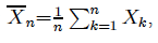 whose distribution in this case is Binomial (Bin):

derived by assuming the validity of the statistical model assumptions ‘BerIID’. Any attempt to use (3) to define any error probabilities, including the p-value (Titelbaum (2022), p. 465), is improper and will give rise to the wrong inference.
A frequentist test comprises two equally important components. For the hypotheses in (2), the optimal N-P test takes the form:

In frequentist testing, the test statistic is always a distance function d(X) framed in terms of a statistic and a frequentist test also includes a rejection region whose choices are neither arbitrary or whimsical. Indeed, the choice of d(X) and C1(α) is interrelated and needs to satisfy two conditions. The first is that the distribution of d(X) can be evaluated under both H0 and H1, and the second is that it has to give rise to an optimal test in terms of learning from data about θ*, and there are good choices for d(X) and C1(α) and bad ones, which are evaluated in terms of their capacity to approximate θ* framed in terms of their pre-data type I and II error probabilities.
In the case of the test in (4), the N-P optimal theory of testing renders it Uniformly Most Powerful (UMP) whose relevant sampling distributions are:

where ‘≈’ indicates an approximation of the scaled Binomial by the Normal distribution; see Spanos (2019).
Example 1. Consider particular data x0 representing 17 Hs out of n=20 flips (Titelbaum, 2022, p. 465):
HHHTHHHHHTHHHHTHHHHH (6)
In light of the fact that this p-value is based on n=20 observations, this indicates a clear departure from θ0 =.5. It is important to emphasize that the p-value in (8) is NOT the probability of the particular configuration in (6) occurring as a realization of the sample!
The question that arises at this stage is ‘what about the validity of the probabilistic assumptions comprising the invoked statistical model in (1) for the particular data x0?’ If any of these assumptions are invalid for x0 the above inference results are unreliable! The Bernoulli assumption is innocuous since any data with two outcomes can always be framed with such a distribution. The IID assumptions, however, are often invalid with real data. When IID is invalid, the assumed distributions under both H0 and H1 in (5) are invalid, inducing sizeable discrepancies between the actual error probabilities and the nominal ones derived by assuming the validity of IID! This renders any evaluations based on their tail areas highly misleading; see Spanos (2019), ch. 15. Hence, in practice one needs to test the IID assumptions before using x0 in the context of the statistical model in question to draw inferences about θ*.
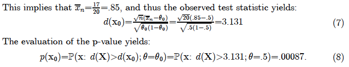
Example 2. Let us return to the particular data x0 representing 17 Hs out of n=20 flips, and ask the question: Are the IID assumptions valid for data x0? Although there are many ways to test the IID assumptions (Spanos, 2019, ch.15), a particularly simple misspecification test is the runs test. A ‘run’ is a segment of the sequence of outcomes consisting of adjacent identical elements which are followed and proceeded by a different symbol. For the observed sequence in (6), the sequence of 7 runs is shown below:

The runs test compares the actual number of runs R with the number of expected runs E(R)— assuming that the sample is IID process — to construct the runs test:
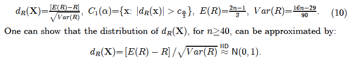
Note that the above runs test can be extended to a more sophisticated test which accounts, not only for the number of runs, but also their different lengths, e.g. run 1 has length 3, run 2 has length 1 and run 3 has length 5.
In this case the sample size n =20, is rather small, but we can apply the test anyway for illustration purposes:

where the p-value indicates departures from the IID assumptions at any significance level α ≥ .032. One can dispute this particular threshold α but in light of the small sample size n=20, this threshold ensures that the test has sufficient power to detect departures from IID. On the issue of why the p-value should always be one-sided is because the data render irrelevant one of the two tails post-data (when dR(x0) is revealed). This is the key difference between the p-value and type I and II error probabilities that are pre-data; see Spanos (2019). ch. 13.
It is important to emphasize that the runs test in (10) is probing the validity of the IID assumptions underlying the invoked statistical model in (1), and thus it poses very different questions to the data when compared to the N-P test in (5) which assumes the validity of the assumptions and probes for θ*! Indeed, misspecification testing should not be framed in terms of the parameter(s) of the underlying statistical model because it probes outside the boundaries of the given model, as opposed to N-P testing that probes within its boundaries. In practice, misspecification testing predates N-P testing to secure the validity of the invoked statistical model and thus the reliability of the ensuing inference; see Mayo and Spanos (2004).
More broadly, the accept/reject H0 results and small/large p-values do not provide evidence for or against particular hypotheses since the sample size n in conjunction with the pre-specified α play a crucial role in transforming such results into evidence using their post-data severity evaluation that outputs the warranted discrepancy from the null value; see Mayo and Spanos (2006). For a given α, ignoring the sample size n is likely to give rise to the fallacies of acceptance and rejection. This is due to the inherent trade-off between the type I and II error probabilities, which implies that for a given α the power of the test increases with n. The post-data severity evaluation provides an evidential account of the accept/reject H0 results by taking fully into account the sample size n; see Mayo (2018), Spanos (2023).
Note 1. The widely held impression that Fisher’s significance testing and N-P testing are two very different approaches is just another misconstrual of frequentist testing. They are not so different! Stating just a point null hypothesis H0: θ = θ0 and a threshold α, Fisher brings into play the type I and II error probabilities (and power) indirectly into his significance testing. Don’t take my word for this claim, read Fisher (1935), pp. 21-22 describing how the power of the test increases with the sample size n but calling it the ‘sensitivity’ of a test. How could one explain the acerbic Fisher vs. Neyman-Pearson exchanges? They were talking passed each other since the type I and II error probabilities are pre-data — framing the capacity of the test —, and Fisher’s p-value is post-data evaluation indicating potential departures from H0 in light of the observed test statistic. Fisher can get away without specifying an alternative hypothesis H1 since the sign of the observed test statistic indicates the direction of departure, eliminating one of the two tails; see Spanos (2019), ch. 13. It should be noted that Fisher constructed his numerous test statistics using intuition, but they turned out to define optimal frequentist tests when supplemented by an appropriate rejection region, and Neyman and Pearson (1933) give him credit for that.
Note 2. For further discussions on frequentist testing, its misinterpretations and misuses, including the base-rate fallacy, the Jeffreys-Lindley Paradox, Akaike type selection criteria, etc., see the following papers:
- Spanos, Aris (2007) “Curve-Fitting, the Reliability of Inductive Inference and the Error-Statistical Approach,” Philosophy of Science, 74(5): 357-381.
- Spanos, Aris (2010) “Is Frequentist Testing Vulnerable to the Base-Rate Fallacy?” Philosophy of Science, 77: 565-583.
- Spanos, Aris (2013) “Who Should Be Afraid of the Jeffreys-Lindley Paradox?” Philosophy of Science, 80: 73-93.
- Spanos, Aris (2022) “Severity and Trustworthy Evidence: Foundational Problems versus Misuses of Frequentist Testing.” Philosophy of Science 89(2): 378-397.
References
[1] Fisher, R.A. (1922) “On the mathematical foundations of theoretical statistics”, Philosophical Transactions of the Royal Society A, 222: 309-368.
[2] Fisher, R.A. (1935) The Design of Experiments, Oliver and Boyd, Edinburgh.
[3] Mayo, Deborah G. (2018) Statistical inference as severe testing: How to get beyond the statistics wars, Cambridge University Press.
[4] Mayo, D.G. and A. Spanos (2004) “Methodology in Practice: Statistical Misspecification Testing”, Philosophy of Science, 71: 1007-1025.
[5] Mayo, D.G. and A. Spanos. (2006) “Severe Testing as a Basic Concept in a Neyman-Pearson Philosophy of Induction”, The British Journal for the Philosophy of Science, 57: 323-357.
[6] Neyman, J. and E.S. Pearson (1933) “On the problem of the most efficient tests of statistical hypotheses”, Philosophical Transactions of the Royal Society, A, 231, 289-337.
[7] Spanos, Aris (2019) Introduction to Probability Theory and Statistical Inference: Empirical Modeling with Observational Data, 2nd edition, Cambridge University Press, Cambridge.
[8] Spanos, Aris (2023) “Revisiting the Large n (Sample Size) Problem: How to Avert Spurious Significance Results.” Stats 6(4): 1323-1338.


")


Aris:
I’m very greatful for your guest post on Titelbaum. The most important point you raise is that testing assumptions corresponds to a different inference than, say, testing the value of a parameter given a model. When Titelbaum says he’s troubled because there are so many different statistics one could use, each corresponding to a different p-value for “the null”, he overlooks the fact that “the null” corresponding to each test is very different. The question being answered, e.g., about an underlying value of theta, is very different than when asking about whether IID holds for these data. The brilliant thing about TEST STATISTICS which are not just any old statistics, is that their distribution is known under the corresponding null hypothesis. Different test statistics correspond to different p-values, as their distributions differ. Wasserstein et al (2016) are blameworthy for defining the p-value in relation to a “summary of the data” without stipulating the requirements for a test statistic. I and others expressed this at the time. Now we have a new generation of practitioners perhaps more confused than the last because most people used to know what’s required for a test statistic (leading to a p-value being uniformly distributed under its corresponding null.)
Aris:
A question for you: Gelman has recently claimed that he would do model checking using graphs without using p-values or similar test statistics. I’m curious if you think graphical analysis suffices. Given your astuteness with such visualizations, you might agree, but I wonder if in general it is feasible to discern model violations in this way. I suppose AI/ML could do it. Of course, the rational and reasoning would still be the same. As Gelman took the lead in abandoning significance and endorsing “no thresholds”, he would defend his use in the context of testing assumptions as being self-critical, or Bayesian p-values. “I’m still interested in model checking (“pure significance testing,” “error probes,” “severe testing,” etc.) but I’m no longer doing this or recommending to do this using p-values.” I can imagine a lot of flexibility in eye-balling data and modifying models.
Deborah: no amount of eyeballing can replace proper misspecification testing for two reasons. First, departures from model assumptions do not arise separately one at a time but always jointly. Hence the use of joint misspecification testing to separate the different departures. Second, eyeballing can take one up to three dimensions, and one would need a ton of observations to see any patterns clearly enough. Looking for patterns relating to several departures form 5 different assumptions in a graph is impossible even with AI! Good luck to Gelman! Thanks for letting me know about the post.
Aris Spanos—Reply to Deborah G. Mayo
I have been using several graphical techniques, including t-plots, scatter-plots, P-P plots, Q-Q plots, histograms, etc., etc., to detect chance regularity patterns exhibited by particular data sets as they relate to probabilistic assumptions in my applied work in econometrics for four decades. I can attest to their effectiveness in guiding a practitioner through model checking or more appropriateness Mis-Specification (M-S) testing to establish the approximate validity of the probabilistic assumptions comprising a particular statistical model invoked for inference purposes using data.
Having said that, let me qualify it by saying that graphical techniques can be excellent in guiding the process of M-S testing. Still, they should never be the final arbiters in deciding whether a statistical model is misspecified or not for a particular data set for several reasons. First, searching for chance regularities patterns relating to several forms of departures from, say 5, different probabilistic assumptions, e.g. an Autoregressive model with p lags [AR(p)], [i] Normality, [ii] Linearity, [iii] Homoskedasticity, [iv] Markov (m) dependence, and [v] constant parameters using only graphs is impossible even with AI! Invariably, departures from model assumptions do not arise separately one at a time, say departures from the Normality assumption, but always jointly. This is because the presence of any form of heterogeneity or/and dependence will invalidate the available Normality tests. Hence the use of joint M-S testing using auxiliary regressions to separate the different forms departures for different probabilistic assumptions. Second, eyeballing can take a practitioner up to three dimensions, and one would need a ton of observations, say more than n=200, to detect any patterns clearly enough. Looking for chance regularities patterns relating to several potential departures from 5 different assumptions using only graphical techniques is impossible even with AI!
For a more detailed discussion of graphical techniques and M-S testing see:
Spanos, A. (2018) “Mis-Specification Testing in Retrospect”, Journal of Economic Surveys, 32(2): 541–577.
Spanos, A. (2019) Introduction to Probability Theory and Statistical Inference: Empirical Modeling with Observational Data, 2nd edition, Cambridge University Press, Cambridge.
This is an interesting post that raises many complex issues. I agree with Aris that the difference between Fisher and Neyman is often exaggerated. Such exaggeration may also be accompanied by a claim that “null hypothesis significance testing” (NHST) is a monstrous chimera. In particular, P-values come in for a lot of criticism and RA Fisher gets the blame. However, Lehmann, surely one of Neyman’s most devoted disciples, advocated the use of P-values and tail area probabilities, and furthermore they had been in regular use in the century before Statistical Methods for Research Workers. This explains why Student, who was a Bayesian (even if the term was not in current use at the time), felt it was important to tabulate the integral of his distribution. Thus P-values not only do not make the difference between the Neyman-Pearson (NP) system and the Fisherian one, they have even been used in certain types of Bayesian application.
I also agree with Aris (of course) that alternative hypotheses are a key feature of the NP system. I am not convinced, however, that they constitute an improvement on Fisher’s approach. As I put it in a blog(1) on this site Fisher’s point of view is “statistics are more primitive than alternative hypotheses and the latter cannot be made the justification of the former”. Furthermore, my view is that the standard interpretation of the famous NP lemma is back to front. Power is not the justification for the likelihood criterion. It is likelihood that is fundamental and power, which is less important, may be an incidental bonus and the lemma explains how. Indeed, where likelihood and power requirements diverge, pursuing the latter at the expense of the former can lead to absurdities. See (2) for an example.
Aris also raises some interesting points about testing assumptions, This raises various issues, including as to whether such procedures, although intended to beneficial, may on occasion be harmful (see (3) for an example) but that would need a separate blog to discuss.
References
(1)Guest Post: STEPHEN SENN: ‘Fisher’s alternative to the alternative’ | Error Statistics Philosophy
(2)S. J. Senn (2007) Drawbacks to noninteger scoring for ordered categorical data. Biometrics, 296-298; discussion 298-299.
(3) S. Senn: Testing Times (Guest post) | Error Statistics Philosophy
Aris Spanos—response to Stephen Senn
I greatly appreciate Stephen’s comments and agree wholeheartedly with his comment that blaming R.A. Fisher for the misinterpretations, misuses, and outright abuses of the p-value is totally misplaced. These confusions and abuses have been created over several decades primarily by uninformed textbook writers, mostly in the social sciences, taking liberties with the formal concepts of frequentist testing, including the p-value, using the well-known alibi of “simplifying” their discussion for their non-mathematical readers (Spanos, 2014, 2021a) and secondarily by Bayesian statisticians deliberately infusing muddiness into the concept and its role in frequentist testing; see Spanos (2021b).
As for blaming Fisher, let us remind our readers that his (1922) paper recast Karl Pearson’s descriptive statistics, into the model-based induction that has dominated frequentist statistics ever since. Singlehandedly, Fisher put forward a more or less complete theory of “optimal estimation” and a theory of significance testing whose optimal component was framed later by Neyman and Pearson (1933) by developing Fisher’s ideas on significance testing built in the context of his concept of a statistical model. Indeed, a ‘good’ (optimal) N-P test begins with an optimal estimator of the parameter(s) of interest. Immediately afterward, Fisher (1934) discussed the optimality of N-P tests (UMP) within his exponential family. His discussion includes the concept of an alternative hypothesis, significance levels, and the power of tests, in a positive tone: “Neyman and Pearson introduced the notion that any chosen test of a hypothesis H₀ is more powerful than any other equivalent test, with regard to the alternative hypothesis H₁, when it rejects H₀ in a set of samples having an assigned aggregate frequency ε [α] when H₀ is true.” (p. 295)
The N-P theory of optimal testing is framed in terms of pre-data error probabilities (type I and II) aiming to calibrate the capacity of the test in detecting different discrepancies from the null value. There is no real conflict with Fisher’s p-value which is a post-data error probability aiming to provide ‘evidence’ against the hypothesized null value by only indicating the presence of “some” discrepancy from that value; Fisher was a falsificationist before Popper (1935) coined the term. Unfortunately, the p-value provides information about the “direction” of the discrepancy but NO information about its “magnitude” since:
The same problem with the magnitude arises with the N-P accept/reject H₀ results. The post-data severity evaluation aims to fill this gap by outputting the “discrepancy” from the null value warranted by the particular data and the test in question with high enough probability; see Mayo and Spanos (2011).
Mayo, D.G. and A. Spanos (2011) “Error Statistics,” pp. 173-208 in the Handbook of Philosophy of Science, vol. 7: Philosophy of Statistics, D. Gabbay, P. Thagard, and J. Woods (editors), Elsevier, 2011.
Popper, Kar (1935) Logik der Forschung, Vienna, Springer.
Spanos, Aris (2014) “Recurring Controversies about P values and Confidence Intervals Revisited,” Ecology, 95(3), 645—651.
Spanos, Aris (2021a) “Revisiting Noncentrality-based Confidence Intervals, Error Probabilities, and Estimation-based Effect Sizes”, Journal of Mathematical Psychology, 104: 102580.
Spanos, Aris (2021b) “Bernoulli’s golden theorem in retrospect: error probabilities and trustworthy evidence.” Synthese 199: 13949-13976.
Stephen:
Thank you for your comment Given your unique position of favoring Fisher to N-P, I’m wondering how you would answer the charge Titelbaum raises about the different test statistics. Most of the ones he mentions are just testing different things, e.g., the value of Normal mean as opposed to testing if ID holds. But in the case of, say, clinical trials (on which you are the expert) testing of a null hypothesis of “no effect”, I wonder where the different choices of test statistic are reflected in the inference reached. Does it suffice to report what was tested (e.g., differences vs ratios)?
I replied to him quoting your earlier guest post.
https://errorstatistics.wordpress.com/wp-admin/edit-comments.php?s=71.171.1.42&mode=detail
I quoted your saying
“All that you can do is apply your experience to use statistics, which when employed in valid tests, reject the null hypothesis most often.” (Senn post)–at least when it is false.
This suggests that the relevant test stat (or the alternative) is arrived at by considering what kind of departure (from the null) allows rejecting it most often. But I don’t know if that’s what you think Fisher would say.
I’d like to get this issue straightened out now that it has come up and I am so fortunate to have you on the other end for a moment. Moreover, I hope to speak at the Neyman seminar at Berkeley soon, and Fisher vs N-P is bound to come up. thank you so much!
Dear Deborah,
Thanks for your comments.
I posted a reply to your comment but it seems to have disappeared.
Regards
Stephen
Colorful basement?
I’ve searched the spam for your comment but don’t see it. I’m sorry. There is a ML bot in charge of comments, they tell me, and it is hard to control. If you can re-enter your comment, I’d be very grateful. Thank you.
My apologies, Deborah. I have no idea where colorfulbasement came from and I wouldn’t even spell colourful that way nor refer to a cellar as basement! I did not keep a copy of my post, so I shall start again.
It seems to me that some pioneering theoretical statisticians had the ambition of creating a single unified theory of inference. I think Neyman fell into this category and, for example, he made his theory of testing also a theory of estimation. I also think he what he was interested in doing was mathematics. Fisher, on the other hand, was interested in science and what he did was create inferential tools: significance tests, likelihood, fiducial inference and, of course a host of techniques that scientists could use for design and analysis, such as randomisation, blocking, analysis of variance, discriminant analysis etc.
So, from Fisher’s point of view, Neyman provides a solution to a mathematical problem that is not a solution to the scientific one. A good example of one of their disputes along these lines is their dispute on the analysis of Latin Squares, where, from Fisher’s point of view, Neyman provides a test fro a Null hypothesis that no-one could believe in. See Added Values for a discussion(1).
So, Fisher’s objection to the Neyman-Pearson system is that one has to make assumptions regarding an alternative hypothesis in order to be able to use such assumptions to justify the particular test chosen. This leaves one with the problem of how to justify one set of assumptions rather than another. A true mathematician won’t care but a scientist will. One could say that what Neyman is doing is no different in kind from assuming that a nuisance parameter is known. Choose a value of the population standard deviation by assumption and then you won’t have to use a t-test.
I think that there is much to be said for Fisher’s criticism but (as he was generally quite happy to do) he takes it so far. I explain why in my post on this site. Guest Blog: STEPHEN SENN: ‘Fisher’s alternative to the alternative’ | Error Statistics Philosophy
Reference
(1) S. J. Senn (2004) Added Values: Controversies concerning randomization and additivity in clinical trials. Statistics in Medicine, 3729-3753.
Stephen:
Thank you so much for your reply. I removed the strange name the machine assigned to you. I only received a reply from the bot running WordPress nowadays.
As I see it, Neyman was called on by Pearson to underwrite, mathematically, Fisher’s choices of tests and intuitively plausible tests, even though Fisher left it open to scientific experience or judgment. A quote from my book SIST says:
Fisher (1935a, p. 187) is well aware that “the same data may contradict the hypothesis in any of a number of different ways,” and that different corresponding tests would be used. The notion that different tests of significance are appropriate to test different features of the same null hypothesis presents no difficulty to workers engaged in practical experimentation. . . . [T]he experimenter . . . is aware of what observational discrepancy it is which interests him, and which he thinks may be statistically significant, before he enquires what test of significance, if any, is available appropriate to his needs.” (ibid., p. 190)
Even if ‘an experienced experimenter’ knows the appropriate test, this doesn’t lessen the importance of N-P’s interest in seeking to identify a statistical rationale for the choices made on informal grounds.”
As for Neyman being more of a mathematician than a scientist, Neyman is very different in his applied work. He talks inferentially rather than behavioristically. There are posts on this blog alluding to what I call “hidden Neyman”. These are papers, discovered by Spanos and I, where Neyman has clearly moved away from his earlier behavioristic self. On the question of who was more rigid on thresholds, Lehmann emphasizes that N-P always suggested balancing errors in relation to context.
Cox (2020) wrote, surprisingly:
“In his later, more applied work, Neyman departed somewhat from that and used p-values flexibly, whereas Fisher paradoxically, in some at least of his work, used 5% significance rather rigidly, although he recognized the arbitrariness of that specific choice.”
As for the example that you mention, it was discussed a lot on this blog. You give a very clear illumination of what’s wrong with Neyman’s model in the discussion to this post.
Gelman claims to agree with Neyman by considering estimation rather than testing:
The big problem I have with taking most of the Fisher-Neyman dispute at face value is that by 1935 they were at each other’s throats for various other reasons…
We are trying to fix the comment approval system. Hopefully soon it will be fixed.
Regarding misspecification testing, our review and discussion paper with a new result presented at Mayo’s earlier series of webinars is now published:
Iqbal Shamsudheen, Christian Hennig (2023) Should We Test the Model Assumptions Before Running a Model-based Test? Journal of Data Science, Statistics, and Visualisation, 3(3). https://doi.org/10.52933/jdssv.v3i3.73
I think that we give a balanced account there, exploring Stephen Senn’s remark that in some situations misspecification testing can be harmful, but also giving some conditions under which choice of a test based on misspecification testing can be expected to work well.
A major issue here is that model assumptions don’t need to be (literally) fulfilled (they never are) for model-based tests to make sense. What we need is that model assumptions are not violated in such a way that they lead to misleading conclusions. This is however a rather subtle criterion that is hard to assess. Unfortunately it can’t be taken for granted that what is in fact needed is that a misspecification test (or, as Aris is always keen to emphasise, a decision rule based on more than one MS test applied in appropriate order) doesn’t reject the model assumptions. There are a number of situations in which MS tests will reject assumptions but the corresponding model-based test will still work well (for example based on very large samples that make tiny deviations look significant, or in situations in which the CLT grants approximate normality of the test statistic even if data or residuals look very non-normal). Depending on the specific situation and MS test protocol, on the other hand, also situations can be found in which there are problematic issues with model assumptions that are not found by the MS tests run. Sometimes (but not always) in such cases, visualisation can help. But of course “eyeballing” will always depend on the analyst who does it, and cannot be formally analysed or even simulated (unless what we do when eyeballing is formalised, amounting to defining another MS test).