

“This is the kind of cure that kills the patient!”
is the line of Aris Spanos that I most remember from when I first heard him talk about testing assumptions of, and respecifying, statistical models in 1999. (The patient, of course, is the statistical model.) On finishing my book, EGEK 1996, I had been keen to fill its central gaps one of which was fleshing out a crucial piece of the error-statistical framework of learning from error: How to validate the assumptions of statistical models. But the whole problem turned out to be far more philosophically—not to mention technically—challenging than I imagined.I will try (in 3 short posts) to sketch a procedure that I think puts the entire process of model validation on a sound logical footing. Thanks to attending several of Spanos’ seminars (and his patient tutorials, for which I am very grateful), I was eventually able to reflect philosophically on aspects of his already well-worked out approach. (Synergies with the error statistical philosophy, of which this is a part, warrant a separate discussion.)
Problems of Validation in the Linear Regression Model (LRM)
The example Spanos was considering was the the Linear Regression Model (LRM) which may be seen to take the form:
M0: yt = β0 + β1xt + ut, t=1,2,…,n,…
Where µt = β0 + β1xt is viewed as the systematic component, and ut = yt – β0 – β1xt as the error (non-systematic) component. The error process {ut, t=1, 2, …, n, …,} is assumed to be Normal, Independent and Identically Distributed (NIID) with mean 0, variance σ2 , i.e. Normal white noise. Using the data z0:={(xt, yt), t=1, 2, …, n} the coefficients (β0 , β1) are estimated (by least squares) yielding an empirical equation intended to enable us to understand how yt varies with Xt.
Empirical Example
Suppose that in her attempt to find a way to understand and predict changes in the U.S.A. population, an economist discovers, using regression, an empirical relationship that appears to provide almost a ‘law-like’ fit (see figure 1):
yt = 167.115+ 1.907xt + ût, (1)
where yt denotes the population of the USA (in millions), and xt denotes a secret variable whose identity is not revealed until the end (these 3 posts). Both series refer to annual data for the period 1955-1989.
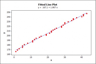
Figure 1: Fitted Line
A Primary Statistical Question: How good a predictor is xt?
The goodness of fit measure of this estimated regression, R2=.995, indicates an almost perfect fit. Testing the statistical significance of the coefficients shows them to be highly significant, p-values are zero (0) to a third decimal, indicating a very strong relationship between the variables. Everything looks hunky dory; what could go wrong?
Is this inference reliable? Not unless the data z0 satisfy the probabilistic assumptions of the LRM, i.e., the errors are NIID with mean 0, variance σ2.
Misspecification (M-S) Tests: Questions of model validation may be seen as ‘secondary’ questions in relation to primary statistical ones; the latter often concern the sign and magnitude of the coefficients of this linear relationship.
Partitioning the Space of Possible Models: Probabilistic Reduction (PR)
The task in validating a model M0 (LRM) is to test ‘M0 is valid’ against everything else!
In other words, if we let H0 assert that the ‘true’ distribution of the sample Z, f(z) belongs to M0, the alternative H1 would be the entire complement of M0, more formally:
H0: f(z) € M0 vs. H1: f(z) € [P – M0]
where P denotes the set of all possible statistical models that could have given rise to z0:={(xt,yt), t=1, 2, …, n}, and € is “an element of” (all we could find).
The traditional analysis of the LRM has already, implicitly, reduced the space of models that could be considered. It reflects just one way of reducing the set of all possible models of which data z0 can be seen to be a realization. This provides the motivation for Spanos’ modeling approach (first in Spanos 1986, 1989, 1995).
Given that each statistical model arises as a parameterization from the joint distribution:
D(Z1,…,Zn;φ): = D((X1, Y1), (X2, Y2), …., (Xn, Yn); φ),
we can consider how one or another set of probabilistic assumptions on the joint distribution gives rise to different models. The assumptions used to reduce P, the set of all possible models, to a single model, here the LRM, come from a menu of three broad categories. These three categories can always be used in statistical modeling:
(D) Distribution, (M) Dependence, (H) Heterogeneity.
For example, the LRM arises when we reduce P by means of the “reduction” assumptions:
(D) Normal (N), (M) Independent (I), (H) Identically Distributed (ID).
Since we are partitioning or reducing P by means of the probabilistic assumptions, it may be called the Probabilistic Partitioning or Probabilistic Reduction (PR) approach.[i]
The same assumptions, traditionally given by means of the error term, are instead specified in terms of the observable random variables (yt, Xt): [1]-[5] in table 1 to render them directly assessable by the data in question.
| Table 1 – The Linear Regression Model (LRM) | ||
|
yt = β0 + β1xt + ut, t=1,2,…,n,… |
||
| [1] Normality: | D(yt |xt; θ) | Normal |
| [2] Linearity: | E(yt |Xt=xt) = β0 + β1xt | Linear in xt |
| [3] Homoskedasticity: | Var(yt |Xt=xt) =σ2, | Free of xt |
| [4] Independence: | {(yt |Xt=xt), t=1,…,n,…} | Independent |
| [5] t-invariance: | θ:=(β0 , β1, σ2), | constant over t |
There are several advantages to specifying the model assumptions in terms of the observables yt and xt instead of the unobservable error term.
First, hidden or implicit assumptions now become explicit ([5]).
Second, some of the error term assumptions, such as having a zero mean, do not look nearly as innocuous when expressed as an assumption concerning the linearity of the regression function between yt and xt .
Third, the LRM (conditional) assumptions can be assessed indirectly from the data via the (unconditional) reduction assumptions, since:
N entails [1]-[3], I entails [4], ID entails [5].
As a first step, we partition the set of all possible models coarsely
in terms of reduction assumptions on D(Z1,…,Zn;φ):
| LRM | Alternatives | |
| (D) Distribution: | Normal | non-Normal |
| (M) Dependence: | Independent | Dependent |
| (H) Heterogeneity: | Identically Distributed | Non-ID |
Given the practical impossibility of probing for violations in all possible directions, the PR approach consciously considers an effective probing strategy to home in on the directions in which the primary statistical model might be potentially misspecified. Having taken us back to the joint distribution, why not get ideas by looking at yt and xt themselves using a variety of graphical techniques? This is what the Probabilistic Reduction (PR) approach prescribes for its diagnostic task….Stay tuned!
*Rather than list scads of references, I direct the interested reader to those in Spanos.
[i] This is because when the NIID assumptions are imposed on the latter simplifies into a product of conditional distributions (LRM).


")


You don’t need to check Normality here. Homoskedasticity is sufficient for valid (frequentist) inference on the beta parameters, given large samples. There are also straightforward large-sample methods that don’t require linearity, or homoskedasticity.
Some other points I hope you will be addressing in future posts;
i) There is only power to diagnose model-misspecification in a finite number of directions (see e.g. Escanciano, 2009, Econometric Theory) – you can’t have power against general alternatives.
ii) The act of preliminary model checking invalidates frequentist properties of tests that ignore this model checking (see e.g. Leeb and Potscher, 2005, Econometric Theory)
iii) Linear models (and much else) can be motivated from arguments of exchangeability and sufficiency alone; see Diaconis and Freedman’s work in the 1980s.
I’m not sure how you define valid inference, but what model validation is aiming to do is to secure the reliability of inference in the sense that the actual error probabilities associated with any inference of interest are close to the nominal (assumed) ones. When one applies a 5% significance level test for the coefficient of x, the actual error probability is close to that value. The fact that one has a Consistent and Asymptotically Normal (CAN) estimator does not guarantee that! Indeed, you qualify your valid inference claim with “given large samples”. The sample size here is n=35. Is it large enough in your evaluation?
i) One can only probe a finite number of directions, but if you use alternatives that partition the set of all alternative models you can eliminate an infinite number of alternatives each time!
ii) The pre-test bias argument, when applied to M-S testing, it is totally misplaced because it amounts to adopting and formalzing the fallacy of rejection as a sound basis for inference; see Spanos, A. (2010), “Akaike-type Criteria and the Reliability of Inference: Model Selection vs. Statistical Model Specification,” Journal of Econometrics, 158: 204-220. This paper includes a reply to the argument in Leeb and Potscher, 2005, Econometric Theory.
iii) Exchangeability imposes highly restrictive forms of dependence and stationarity on the stochastic process underlying the data, and it is not particularly realistic for most data in economics. Moreover, motivating a model and securing the reliability of inference based on such a model are very different objectives.
AS: thanks for weighing in here. As I’m sure you’re aware, the issue of what n is “large” is a red herring. If one wants to check the accuracy of approximations, one does simulations under plausible truths. If one can’t live with this degree of approximation (which may be defensible in some applications) then one should answer questions that only permutation-based inference can address, and should *not* use methods like e.g. logistic regression, that provide only approximate inference even when the underlying model is entirely accurate. Let’s not have the perfect be the enemy of the good.
i) Blocking like this dilutes the effect of the model-deviation you presumably want to detect; there may still be little power to detect deviations. If you’re then happy to conclude that we just can’t perform a severe test, fine – but this is not what users conclude in practice, see my reply to Mayo.
ii) If it messes up the error probabilities, by your definition of what model validation is aiming to do, then we still have a problem.
iii) I totally agree about exchangeability in econometrics. In other situations it is however highly plausible, and sufficiency of low-dimensional statistics is a natural desiderata of analysts. That these together can imply e.g. “Normality + a prior” suggests other ways to motivate models, quite unlike postulating error processes; these methods need not be bound by the same model-specification issues discussed here.
Link to working paper version of Akaike-type Criteria and the Reliability of Inference: Model Selection vs. Statistical Model Specification.
Of course this was just an illustration….the subtle points are yet to come …
I just noticed what “Guest” wrote in (ii): that’s absurd and completely false–please spell out their argument, or alleged argument. It’s the opposite. The correct error probabilities are threatened by failed assumptions.
Mayo: It’s not absurd, nor is it false. It’s not even unusual. If we choose to use e.g. an equal-variance or unequal-variance t-test based on a “pre-test” for e.g. equal variance, then the overall Type I error rate of the result is not preserved – at least by the naive analysis that ignores the pre-test. Yet this is *exactly* what many textbooks and instructors tell users to do.
The same problems occur when pre-testing for Normality, or any form of pre-testing which is not independent of the actual inference of interest.
I agree that failed assumptions lead to incorrect results, but we need to be careful about i) precisely which assumptions cause the trouble ii) what we mean by “incorrect”, which in testing involves stating the null hypothesis rather precisely, and iii) realizing that even well-intentioned pre-tests are capable of doing more harm than good.
Guest: I maintain the argument to which I believe you are alluding is wrong; you haven’t given the argument, but I’m guessing it’s that very old fallacy.* I’m glad we’ll get to straighten out some confusions surrounding these issues over the next few weeks. Sorry I’m in between jitneys at the moment.
*I qualified this, now that I am in one place, more or less. Alternatively something’s going on in the special case you might have in mind in alluding to pretests being dependent on the inference? Describe.
http://bit.ly/ycriN8
On the issue of pre-test bias as it pertains [or rather it doesn’t] to M-S testing I have already replied to the Leeb and Potscher, 2005, Econometric Theory cited by the guest, in my published paper Spanos, A. (2010), “Akaike-type Criteria and the Reliability of Inference: Model Selection vs. Statistical Model Specification,” Journal of Econometrics, 158: 204-220.
For an earlier version of that discussion see section 6.3 of my working paper version given in the Link by Corey, entitled:
6.3 M-S testing/respecification and pre-test bias
Guest: I think at least one reason we’re talking past eachother is that the paper you cite and others are considering error probabilities that could result from inferring a specific alternative in m-s testing—illegitimate from our perspective (see the Durbin Watson discussion). That said, I might note that, in general, severity associated with inferring a statistical inference is not a matter of long-run error rates of procedures or combined procedures. You might be interested in some of my discussions on double counting and the “selection effections” section in Mayo and Cox (2010). In the realm of m-s testing, the issue is often taken up by Spanos.
I only start to go through this series of postings now, so hopefully this is not too late to be seen.
Anyway, a quick remark. I don’t agree with this bit:
“Is this inference reliable? Not unless the data z0 satisfy the probabilistic assumptions of the LRM, i.e., the errors are NIID with mean 0, variance σ2.”
And I think that you are not precise here about what you think yourself.
Of course we *know* that the normality assumption is not perfectly satisfied in such a situation without any testing, because negative values are possible under a normal and the set of natural numbers (we’re talking about a population size here!) has a probability of zero under any normal distribution.
If “validating the model assumptions” can ever have a useful meaning, it must be something else than “check whether the assumptions are really satisfied”. They are not and we know this, and any real information that comes from model checking tells us something else than that, namely (hopefully) that what we *do* with the model assumption (which is not “true” in any case) addresses a research question properly and is not misleading.
Establishing statistical adequacy [model assumptions [1]-[5] are valid for the particular data] is not about “truth” [whatever that might mean] but error-reliability of inference. That is, it provides an answer to the question “could the process postulated by this model have generated this particular data, on pragmatic grounds. If the answer is yes, it means that the actual error probabilities approximate closely the nominal ones to render any inferences based on the estimated model reliable, statistically speaking, i.e. statistical adequacy is the price one needs to pay to ensure the credibility of the statistical inference invoked. Whether the estimated model sheds adequate light [describes, explains, predicts] the actual phenomenon of interest has to do with the substantive adequacy of the model in question. Conflating the two types of adequacy has given rise to numerous misleading claims in statistical modeling and inference, including the famous slogan “all models are wrong, but some are useful”. In general, if any of the model assumptions [1]-[5] are false one should expect some discrepancy between the actual and nominal error probabilities. Of course not all assumptions are created equal; departures from certain assumptions have more devastating effects on the relevant error probabilities than others. However, when a modeler invokes generic robustness claims such as “small departures from Normality” will not affect the reliabilit of inference too much”, the onus on the modeler to quantify “small depatures” and “too much”. The statistics literature on “robustness” is satiated with misleading claims, primarily because it does not focus its claims on the discrepancy between actual and nominal error probabilities. For those interested, I discuss these issues in detail in Spanos, A. (2009), “Statistical Misspecification and the Reliability of Inference: the simple t-test in the presence of Markov dependence,” The Korean Economic Review, 25: 165-213.
Click to access Spanos-Inference&reliability-2009.pdf
Aris, OK, I see your point and I think that to some extent I agree with it. However, I think that one could be more precise in this respect.
Whether and to what extent error probabilities are affected by violations of the nominal model assumptions depends on what is done with the model later.
In most standard situations it is not a problem that a normal distribution is used to model a situation in which the data can only be natural numbers in a certain finite range, but one can imagine situations in which it is a problem (for example, if tail probabilities are used).
I still think that it is misleading wording to say that model assumptions have to be “satisfied” (actually Mayo says it in a better way in the third part of this series). It may well be that one could say it in a way we could agree on, although for me how model checking should be done should depend on research aims and on what is done with the model later, and what “on pragmatic grounds” means could and perhaps should be made more precise.
By the way, Aris, your linked paper, interesting as it is, doesn’t address the major proponents of robustness theory, such as Huber, Hampel and his co-authors, Davies etc., who I believe are not prone to the mistakes that are specifically criticised in the paper (although you may criticise them for other reasons ;-).
By the way, I agree with the guest technically on point ii of the first posting (I know that Aris can come up with *some* setups in which this isn’t the case but usually it is), but if we acknowledge what I wrote above namely that “making sure the model is true” is not what the checking business is about anyway, the fact that checking often violates the assumptions itself doesn’t mean that it shouldn’t be done.
The key point I tried to make in my 2009 paper is that one cannot usually disentangle clearly vague departures from the model assumptions and their potential distortion of the relevant error probabilities for several reasons.
First, the model assumptions are interrelated, the detected departures are not often very specific and they usually concern more than one assumption in practice. Hence, the claim “departures from Normality that retain the symmetry of the underlying distribution are unlikely to affect the error probabilities of the t-test “too much”, can be very misleading; I can easily produce realistic counterexamples!
Second, to be able to make quantifiable claims about the relevant error probabilities one needs to determine the specific nature of the departure. But if one goes this extra mile, and finds out that, say the underlying distribution is much closer to the Uniform rather than the Normal, the t-test is the wrong (non-optimal) test to apply!! There is a much better test to use in the context of a respecified Uniform IID model that I discuss in my 2009 paper.
I can go on and on, on how misleading certain widely-used generic robustness claims can be in practice, but I will not!
In relation to the traditional robustenss literature, as discussed by Huber, Hampel etc., my point is that they do not focus their discussion on the discrepancy between the actual and nominal error probabilities, which is, in my view, the best way to assess the error-reliability of frequentist inference. Hence, some departures that are evaluated as serious in the traditional context turn out to be approximately okay in terms of the relevant error probabilities and the other way around! This is primarily due to the fact that the traditional literature on robustness focuses primarily on discrepancies between different models, and “big” and “small” discrepancies in that context do not necessarily translate into “big” and “small” discrepancies between the actual and nominal error probabilities.
The “robustniks” cited by me certainly don’t claim that the t-test is robust… At least Huber’s classical robustness theory is about the distributions of estimators in neighborhoods of the nominal model, which is not directly about error probabilities, but they could be derived from such a theory. You should be able to find some work about robust inference, too, that considers error probabilities. Although it may be true that the robustniks focus more on estimation theory and less on error probabilities than one would like.
Regarding optimality, the more realistic situation is that one could think about the underlying distribution as neither exactly Gaussian nor uniform nor Cauchy, and even if you can figure out that it looks clearly closer to one of them than to the others (closest to the uniform, say) it is far from clear that a test that is optimal under the uniform will still be better than those derived from other assumptions under the actual distribution that is “similar” to the uniform but not equal. And this is one of the (as far as I think) highly relevant contributions of robust statistics, that you ask, is it really true that something that is optimal under a certain nominal model is still good (if not optimal) in a neighborhood of “similar” distributions – and often it is not, and one rather may choose something that, for example, is optimal in a minimax sense over a full neighborhood of distributions.
Christian, AS; to invalidate the (unequal variance) t-test under independence you have to go a long way into heavy-tailedness, and/or small sample size. These concerns may be entirely appropriate in discussions of e.g. modest amounts of cost data – but such “counterexamples” are not uniformly realistic.
Also, in discussing robustnik methodology etc – which I agree is relevant – it’s important to distinguish robustness to particular data points from robustness to particular modeling assumptions. These are not the same thing, one can have either/or/neither/both.
guest: The type II error probability (power) of the t-test can certainly be broken down quite easily (a single outlier will do), though it’s a more difficult business for the type I error probability.
The second remark is correct, although these are closely related as you probably know.