
 Stephen Senn
Head, Methodology and Statistics Group,
Competence Center for Methodology and Statistics (CCMS),
Luxembourg
“Dawid’s Selection Paradox”
You can protest, of course, that Dawid’s Selection Paradox is no such thing but then those who believe in the inexorable triumph of logic will deny that anything is a paradox. In a challenging paper published nearly 20 years ago (Dawid 1994), Philip Dawid drew attention to a ‘paradox’ of Bayesian inference. To describe it, I can do no better than to cite the abstract of the paper, which is available from Project Euclid, here: http://projecteuclid.org/DPubS/Repository/1.0/Disseminate?
When the inference to be made is selected after looking at the data, the classical statistical approach demands — as seems intuitively sensible — that allowance be made for the bias thus introduced. From a Bayesian viewpoint, however, no such adjustment is required, even when the Bayesian inference closely mimics the unadjusted classical one. In this paper we examine more closely this seeming inadequacy of the Bayesian approach. In particular, it is argued that conjugate priors for multivariate problems typically embody an unreasonable determinism property, at variance with the above intuition.
I consider this to be an important paper not only for Bayesians but also for frequentists, yet it has only been cited 14 times as of 15 November 2013 according to Google Scholar. In fact I wrote a paper about it in the American Statistician a few years back (Senn 2008) and have also referred to it in a previous blogpost (12 May 2012). That I think it is important and neglected is excuse enough to write about it again.
Philip Dawid is not responsible for my interpretation of his paradox but the way that I understand it can be explained by considering what it means to have a prior distribution. First, as a reminder, if you are going to be 100% Bayesian, which is to say that all of what you will do by way of inference will be to turn a prior into a posterior distribution using the likelihood and the operation of Bayes theorem, then your prior distribution has to satisfy two conditions. First, it must be what you would use to bet now (that is to say at the moment it is established) and second no amount of subsequent data will change your prior qua prior. It will, of course, be updated by Bayes theorem to form a posterior distribution once further data are obtained but that is another matter. The relevant time here is your observation time not the time when the data were collected, so that data that were available in principle but only came to your attention after you established your prior distribution count as further data.
Now suppose that you are going to make an inference about a population mean, θ, using a random sample from the population and choose the standard conjugate prior distribution. Then in that case you will use a Normal distribution with known (to you) parameters μ and σ2. If σ2 is large compared to the random variation you might expect for the means in your sample, then the prior distribution is fairly uninformative and if it is small then fairly informative but being uninformative is not in itself a virtue. Being not informative enough runs the risk that your prior distribution is not one you might wish to use to bet now and being too informative that your prior distribution is one you might be tempted to change given further information. In either of these two cases your prior distribution will be wrong. Thus the task is to be neither too informative nor not informative enough.
However, as I pointed out in my previous blogpost on this topic, a conjugate prior distribution is perfectly informative about itself. Consider the accompanying figure. Here I have simulated a number of true population means (that is to say possible values of θ) from the prior distribution that governs the probability with which they will arise. (I have chosen a Normal distribution with mean μ=0 and variance σ2 = 25 but any values would do to illustrate the point.) I have simulated 10, 100, 1000 and 10,000 samples from this distribution and in each case the simulated values are shown along the X axis and an empirical density estimation is show as a black curve. For each of the four cases the red curve shows the parent distribution from which the values are simulated.
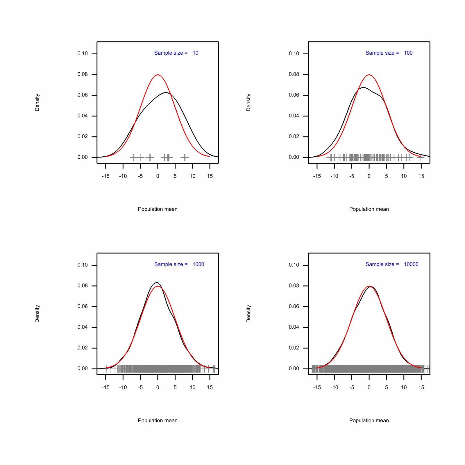
Figure. Empirical density estimates for four different sample sizes
If you look at the empirical density curves you will see that for the samples of 10 and 100 means these do not estimate the distribution well and one could argue that even the sample of 1000 does not do an excellent job although it provides a fair fit. Thus to have a prior distribution is equivalent to having seen rather a lot of information of a certain sort. Note that what the simulation has provided is a sample of true means not sample means, since it is sampled from the prior distribution. Thus the information is equivalent to having seen a very great number of extremely large samples, each from randomly chosen populations from a hyper-population.
Thus, one can see that if this inferential set-up is assumed to apply, the ‘paradox’ becomes explicable. Suppose that you have run a number of experiments measuring (say) ten treatments in vitro. A sample mean is estimated for each of the ten treatments based (say) on 20 replicates. You now choose the largest observed mean and make an inference about the relevant treatment. Why should the fact that this is the largest of ten have any influence on your inference? After all you have a prior distribution that provides information on 1000s of treatments measured using enormous sample sizes. The information provided by the other nine treatments you studied now is paltry by comparison.
But there is a sting in the tail. If I tell you that I took 200 replicates from one treatment and randomly split these into ten samples of 20 and that the mean I am using to make an inference about that treatment is the highest of the 10, then this is something that as a Bayesian you must take account of. In the case of the ten treatments, given the conjugate prior, the distribution of one set of 20 values is conditionally independent of all the other sets. There is no possible leakage of information from one to the other. This is not the same when you are sampling from the same treatment.
This suggests that a way that you can partially restore the frequentist intuition to the Bayesian analysis is to use a hierarchical modelling set up with a hyper-prior distribution on the prior distribution. See my paper for further discussion (Senn 2008).
Note, that I am not claiming here that the frequentist approach is right and the Bayesian is wrong. I am making a point that I have made elsewhere, namely that thinking about each is useful (Senn 2011).
References
Dawid, A. P. (1994). Selection paradoxes of Bayesian inference. Multivariate Analysis and its Applications. T. W. Anderson, K. a.-t. a. Fang and I. Olkin. 24.
Senn, S. (2008). “A note concerning a selection “Paradox” of Dawid’s.” American Statistician 62(3): 206-210.
Senn, S. J. (2011). “You may believe you are a Bayesian but you are probably wrong.” Rationality, Markets and Morals 2: 48-66.


")


Stephen: Thanks so much for the guest post. I’ll study it more tomorrow.
When you say “you have a prior distribution that provides information on 1000s of treatments measured using enormous sample sizes” you seem to be assuming some kind of empirical frequentist prior. Where would the priors on the priors on the priors ever stop?
“Where would the priors on priors on priors ever stop?”
I love it when I can give a a crisp answer to a rhetorical question. The answer is: it need never stop!
That link points to a paper that gives a complete answer with rigor. Here’s a baby version:
Consider a hierarchical sequence of normal distributions of length N. By “hierarchical sequence of normal distributions” I mean that the mean at level i is a random variable with probability law given by the distribution at level i + 1. (This is a specification of conditional distributions; we will be asking questions about the resulting marginal distributions.) Further, suppose the variances are arbitrary. What can we say about the marginal *precision* (inverse of the variance) at the bottom of the hierarchy?
For the normal distribution, the marginal variance is the sum of all of the variances in the hierarchy. As N increases without bound, the sum of the variances could converge or diverge to infinity; the marginal precision must converge, and if the marginal variance diverges, the marginal precision converges to zero. In this situation, none of the marginal distributions in the hierarchy is converging to a proper probability distribution.
Now suppose we use a this tower of distributions as a prior. We start by considering finite N, obtain the posterior, *and then* we consider *convergence of the posterior* as N goes to infinity and the sum of conditional prior variances diverges. The standard analysis applies: the posterior is normal with precision equal to the sum of the prior precision and the data precision, and mean equal to the precision-weighted average of the prior mean and data mean. In the limit as the prior precision goes to zero, we obtain the standard “non-informative prior” result.
Deborah: the point is that to establish a conjugate prior for this case you do three things 1. State the mean 2. State the variance 3. State that it’s Normal.
The problem is that people overlook the fact that 3 is a statement that contains a great deal of information. What is a Normal distribution? Nobody has ever seen one, nor could they. It’s a mathematical idealisation and this idealisation carries more information than a set of observed values ever could. This is the point of the four pictures. The red curve in the four diagrams represents what the Bayesian claims (s)he knows a priori. Suppose I could wipe that Bayesian memory clean and replace the prior distribution in all three of its aspects, knowing the mean, knowing the variance, knowing that it’s Normal, by a sample from the prior distribution, how big would that sample have to be to provide the same information that was in the now erased prior?
Looked at this way you can see that having a prior distribution even if it is vague about the particular mean about which one wishes to make an inference (because its variance is large) is very informative about other matters.
Stephen: Sure, but I imagined that some Bayesian might deny their priors were intended to capture the empirical frequency distributions of parameter values*.
Anyway, how would you state the rationale for caring about the fact that you’re reporting just the treatment that did the best–say for a frequentist.
*By the way, are the assumed priors on each of the 10 treatments or on all treatments, or? Sorry if I missed where you said this.
Well whether you regard the prior distributions as pure mental constructs or empirically based is irrelevant as soon as you start to be Bayesian. the point is that the prior distribution and the likelihood are exchangeable to a degree defined by the model. So prior information behaves as if it were data.
As regards the posterior inference you can regard it as an identification problem. You have a collection of hundreds of thousands of presumed true means making up your prior distribution. You now have an observed mean. Your task is simply to assign a probability that each of these huge numbers of prior means produced the observed mean that you have. Given these probabilities you can construct the probability that the true mean that gave rise to your observed mean lies within any interval whatsover.
Stephen: I’m not sure whether you argue against Bayesian statistics or against a Bayesian hypothesis of mind… If you argue against a Bayesian hypothesis of mind I see your point, how possibly could a perfectly Bayesian agent know that she is measuring something normally distributed without having sampled it 10,000 times first? If you argue against Bayesian statistics, I don’t see your point. Is a Bayesian statistician is a perfectly Bayesian agent with unlimited time and resources? Nope. She has to make modeling assumptions that she doesn’t know are true (or rather that she knows ain’t true) but that might work reasonably well for a particular purpose. If she later on comes up with a modeling assumption that works better (let’s try a t-distribution!) then she could do model comparison, and so on… Maybe this isn’t what you call “100% Bayesian” but who is then? I would still call her “100 % Bayesian statistician” 🙂
As with many paradoxes I don’t really see how this is really a paradox, at least not for Bayesian statistics.
Rasmusab: One of my problems is understanding what it means to say the prior was wrong. Was I wrong about my betting behavior? wrong about the empirical frequency distribution of parameters? or something else?
The meaning of wrong or violated assumptions is much more straightforward (at least for a frequentist error statistician).
Above I was talking about the assumed distribution of the data, not the prior on the model parameters. I agree that it is a bit strang to say that a prior was wrong. Though I guess you could say that it was ill-informed if it didn’t incorporate information that you should have considered or should have known in advance.
Mayo: We can say that the analysis prior is wrong when it forces an inference we (poor saps trying to perform an analysis) know (on the basis of the available prior infomation) to be wrong.
Corey: That still doesn’t tell me what it means for it to be wrong. Senn’s prior was presumably based on the available prior info.
And yet if we find that such a prior forces an inference we judge “wrong”, we ought to be able to point to something in that available prior info to justify that judgment — something that the analysis prior failed to capture.
Rasmusab: I think that it is a dilemma. It is not clear to me whether a Bayesian should or should not worry about the fact that that the mean being the largest of 10 does not change the inference. if you have a single level of prior it doesn’t, if you have more than one level it does.
As regards model-checking, I am not arguing against it but it has to be recognised that it’s a problem for Bayesians and frequentists alike if having checked and established a model you then behave as if you always knew it was true. A further point is that it is not clear that checking itself is a Bayesian activity. The claim that it was something rather different was made very vigorously by George Box.
On a practical level, I think that the paradox is useful in that encourages would-be Bayesians to think a little carefully about their priors. In Senn (2011), cited above, I gave some examples showing how tricky this can be.
Stephen: This should have something to do with how Bayesian statistics is interpreted. Phil Dawid is a de Finettian, as far as I know. Now de Finetti would object to your saying that having a normal prior distribution with known mean and variance implies that you *know* as much as had you seen infinitely many means of samples. In his interpretation the prior distribution does not express distributional knowledge about any “true mean”, which according to him doesn’t exist, but is rather a technical device to express uncertainty about observations to be observable in the future.
It may well be that somebody who is 100% de Finettian (which Dawid is probably not and maybe not even de Finetti himself was always) would argue that the problem/paradox only arises because the analysis is used to make inferential statements about a supposedly true parameter which doesn’t really exist, whereas if the posterior is only used for predicting future observations, there is no problem with using any posterior you might have stopping for whatever reason at whatever point (which doesn’t imply that there is nothing to say about better or not so good ideas about when to stop; this may not influence the validity of the posterior once you have it, but rather your chances of ending up with a useful one).
It is still interesting to look at the implications of the fact that this is formally the same as knowing infinitely many sample means if the prior is interpreted in some kind of frequentist way though…
Christian:
The “true mean” may not exist, even as an adequate model*, but then neither does your true betting odds**, or your actual uncertainty about observations or about anything else. As we’ve seen before, this addled verificationist philosophy refutes itself, since its assertions are non-verifiable. Will we ever take leave of positivistic fetishes?
This reminds me, didn’t de Finetti refuse to assign priors to priors? Then he couldn’t employ Senn’s hierarchical move.
*of a data generating mechanism
**even as an adequate idealization of your uncertainty-generating mechanism
Christian, usually I agree with you but here I don’t. There is no difference in the De Finetti form of Bayesian between a parametric statement and a statement of predictions. The latter follows inevitably from the former. It is just that DeFinetti regards the latter as being a more fruitful and checkabale way to understand things. The point is that the ‘paradox’ does not go away by moving from parametric to prediction space if I may put it thus. The paradox exists because a conjugate prior yields one inference and a hierarchical one another. You need to tell me which you prefer. If you are going to argue hierarchical then I can show you a ton of Bayesian practice that is wrong. If you argue conjugate then I am not sure that Philip Dawid would agree with you. Certainly I think Jack Good would not have done so.
Let me remind you that by using the words “It may well be that somebody who is 100% de Finettian…” I didn’t mean that I am such a person, so I’m not going to defend this position here.
Actually I see now that Stephen is right anyway and I was wrong even from de Finetti’s point of view – stopping rules may influence prediction in equally undue ways they influence inference about unobservable parameters.
Stephen: I just noticed this remark of yours: “If you are going to argue hierarchical then I can show you a ton of Bayesian practice that is wrong.” Can you explain? thanks. Mayo
When you choose a model, you decide what the form of any data used will be, so the conjugate prior is a posterior with respect to information about the form of the data, but not its value. Since this information assumes a particular model chosen out of infinitely many possible ones, I’d say the conjugate prior being equivalent to a large number of samples is an effect of models being underdetermined. It would then be expected that such a prior is “equivalent to having seen rather a lot of information of a certain sort”.
Professor Senn: Why utilize a prior on 1000s of distinct treatments as opposed to priors on the 10 treatments of interest?
Contunuous or discrete it makes no difference. There is only one probabilty distribution. It’s the prior probability for any true mean, including the 10 we happend to have observations on. The red curve is the prior distribution. By integrating this curve between two values you can give the probability that the true mean lies between two limits. But you can regard the continuous distribution as an idealistic representation of large discrete distribution.
Philip Dawid is too busy traveling at the moment to respond to Senn, but here’s the “bon mot” he sends us (upon my request):
“My ‘bon mot’ (straight from the New Orleans French Quarter) would be to emphasise the point that, in problems where we select the parameter of interest after looking at the data (especially when that selection involves some kind of optimisation), the sensitivity of Bayesian inference to the choice of prior can be enormously inflated. An uncritical (e.g., conjugate) formal choice may then to lead to formal posterior inferences you simply should not believe.
Philip”
Stephen: Philip’s bon mot is interesting, and I’m hoping you (and other readers) will consider responding in his place: why, specifically, (i.e., on what grounds) ought you not to believe your formal posterior. Would you say the rationale is frequentist, or something more informal?
And is it that you ought not to use it as your betting odds? or that the posterior doesn’t reflect the actual evidence one has in the data-dependent parameter?
I interpret Philip as meaning this. Whereas for a certain class of problem where the data have arrived without “side” a semi-automatic Bayesian approach may yield inferences that are not too different from what a more careful Bayesian approach might show, this is not so in more complex cases. Here using conventional prior distributions can lead to inferences that will not reflect what the statistician believes.
Stephen: Thanks for broaching this. I was just hoping the learn, specifically, why the selection information would/should alter what the statistician believes. I think that might be very revealing (in connecting the frequentist/Bayesian assessment).
It boils down to this. The probability of a probability is a probability. There are thus some simple cases in which adding levels of a hierarchy changes nothing but in other more complex cases this is not so.
If all the means are drawn from the same (effectively infinite population) then any sample mean is only informative about its own true mean and nothing else. Knowing that it is the largest of the local group is uninformative about anything . However if we have a hierarchical model in which the local group mean is itself drawn from a larger population then any group mean is informative not only about its own ‘true’ parameter value but also about the true mean of the group to which it belongs. This is dicussed in my AmStat paper.
As regards other points that Philip raises, I think this means that the formal Bayesian analysis is nested within some more general informal (also Bayesian) framework that if necessary can check and correct it. I have described this elsewhere as requiring that the informal comes to the rescue of the formal. This is not entirely satisfactory but it is probably realistic and it is what applied statisticians of any inferential religion will recognise as being what they do.
For an example where a conventional frequentist approach comes to grief see
Senn S. Lessons from TGN1412 and TARGET: implications for observational studies and meta-analysis. Pharmaceutical statistics 2008; 7: 294–301.
Stephen: I think I’ll have to leave this as a mystery (to me) again, but I appreciate your efforts to explain. (It’s the rationale I’m after.)
You mention the informal rescuing the formal in your comment. I recall this in a passage in your excellent RMM paper (“You may believe you are a Bayesian but you are probably wrong”.)
“Appeal to a deeper order of things—a level at which inference really takes place that absolves one of the necessity of doing it properly at the level of Bayesian calculation. This is problematic, because it means the informal has to come to the rescue of the formal…..the only thing that can rescue it from producing silly results is the operation of the subconscious.” (Senn, pp 58-9 http://www.rmm-journal.de/downloads/Article_Senn.pdf)
As for the current example, if different Bayesian answers accrue depending on how many iterations of priors one considers, and if the frequentist result (which considers no priors at all) is indicative of the preferred result (even for a Bayesian?) then that would appear to be quite a strong warrant for preferring the frequentist result. But I’m still after the Bayesian rationale for preferring the predictions from whatever hierarchy matches the frequentist inference (whether subconscious or conscious).
Details, complete with illustrative simulations are given in the AmStat paper cited.
It is far too strong to conclude from this example that in general Bayesian approaches, have to be calibrated until they agree with frequentist ones. In the TGN1412 example I cited, for example one could argue the opposite. It is the Bayesian analysis that shows that a naive frequentist one is inappropriate.
I prefer to see it so: when looking at a given problem, try some different frameworks, even if you strongly prefer one. If they disagree, it may suggest that some digging to reveal hidden assumptions is necessary.
All I want are reasons, rationales, even if relative to goals and background. Why strongly prefer? why inappropriate? I keep digging for the same thing (from rare Senn-sible experts) and not quite finding it. Some clues emerge (e.g., as with Dawid’s “bon mot”) and then they slip away… I’ll study your paper, thank you.
Inappropriate because if A Bayesian, knowledgeable, about drug development is forced to think about it (s)he will be forced to admit that the structure of the appropriate prior distribution is (in this case) more complex that that of a conjugate.
Let me give you an analogous situation where a frequentist is forced to think about this also.
Suppose I tell that you a sample of 100 diastolic blood pressures has been taken from a given population. What can you tell me about the DBP in the population? A simple model MODEL 1 is DBP_i = mu +epsilon_i, i=1 to 100 with the epsilon_i of equal variance and independent.
However if I tell you that there are not 100 individuals involved but 20, each of whom has been measured 5 times, then this model won’t do and you need something like MODEL 2
DBP_ij=mu + phi_i + eta_ij, i=1..20, j=1…5. MODEL 1 won’t give you the right answer.
However, the reverse is not a problem. If all along you were using MODEL 2 then MODEL 2 reduces to MODEL 1 if you only have one measurement per subject. In that case epsilon_i = phi_i + eta_i1, and there is nothing in the data that you have that will allow you to make separate statments about any aspect of phi_i + eta_ij, You can only say something about epsilon_ij. (By the by, failure to appreciate this simple fact is one of the reasons why much of what has been said about pharmacogentics is ignorant hype 1- 3.)
So what this shows is that approaches to modelling that work in some cases don’t in others. The selection paradox is a similar example. There are cases where non-hierarchical prior distribution work fine and there are cases where they don’t.
References
1. Senn SJ. Individual Therapy: New Dawn or False Dawn. Drug Information Journal 2001; 35: 1479-1494.
2. Senn SJ. Turning a blind eye: Authors have blinkered view of blinding. BMJ 2004; 328: 1135-b-1136.
3 Dworkin RH, McDermott MP, Farrar JT, O’Connor AB, Senn S. Interpreting patient treatment response in analgesic clinical trials: Implications for genotyping, phenotyping, and personalized pain treatment. Pain 2013.
I never imagined denying that “approaches to modelling that work in some cases don’t in others”, with different info and distinct questions. All I want to know is what you mean by “working” and how you can tell. At times you make is sound as if everyone has enough of the same standpoint to concur about this. I’d even be satisfied to know why, given the goals of school #1, this works great, but not if the goal is #2. You can always tell, and I believe you. I wasn’t asking in general, but just with respect to the case at hand….but anyway, I very much appreciate the discussion and will read about the blinkering business.
In the particular example I gave Model 1 doesn’t work for the case with 20 patients measured 5 times because it produces a variance of the mean that is sigma^2/100, which would only work if the observations were independent, which they are not.
So how can I tell? Well, by having sufficient experience and understanding of the problem to see the issue but also, and this is partly a matter of luck, by not overlooking critical features of the problem.
More generally the point is that all models are based on assumptions (frequentist) or beliefs (Bayesian). These assumptions/beliefs are sometimes critical and sometimes not and if one is not careful one can use a model in a new context without criticising the assumptions/beliefs anew. Here by ‘working’ I mean that not only the assumptions seem reasonable and the logic of the calculation seems right but that the results seem reasonable also.
In a sadly neglected paper(1) I wrote 15 years ago or so, I pointed out that mathemeticians could make bad statisticians if they carried over the habit being formal about everything they did. In particular axiom worship can be a bad habit, a mathematical attitude being “it’s my right to make any assumptions I like and examine the consequences”. In that paper I wrote “models (and even axiomatic systems) are sometimes examined more fruitfully
in terms of their consequences rather than their assumptions.”
de Finetti has a finely expressed comment on a certain type of mathematical attitude:
“In the mathematical formulation of any problem it is necessary to base oneself on some appropriate idealizations and simplification. This is, however, a disadvantage; it is a distorting factor which one should always try to keep in check, and to approach circumspectly. It is unfortunate that the reverse often happens. One loses sight of the original nature of the problem, falls in love with the idealization, and then
blames reality for not conforming to it” (2).
So, in short, it’s really quite difficult to be formal about the business of knowing when models are ‘working’.
1. Senn SJ. Mathematics: governess or handmaiden? Journal of the Royal Statistical Society Series D-The Statistician 1998; 47: 251-259.
2. de Finetti BD. Theory of Probability (Volume 2). Wiley: Chichester, 1975.
Stephen: I seem to remember that paper of yours, so now I have to back and look at it. Too bad that DF fell so in love with his own idealization…
I wouldn’t characterize violated assumptions as a matter of frequencies, or beliefs (except if every darn human assertion is required to have superfluous prefaces: “I believe that” or “I judge that I believe it’s plausible that” ). But there’s no frequency either (at most there might be frequentist implication).
It suffices to say what you mean: “it produces a variance of the mean that is sigma^2/100, which would only work if the observations were independent, which they are not”.
But I’m not sure if the original point in the post about taking the selection aspect into account is also a claim like this. If it is, that should have been the focus (and not whether some hierarchical approach could get the right/reasonable numbers).
The point is that a hierarchical prior allows the fact that the mean chosen is the largest of a number of means to have an impact on the inference. The conjugate prior does not. Similarly, in the example of the blood pressures, Model 2 permits one to take account of the fact that one has repeated observations on the same individual but Model 1 does not. There is a close parallel between the two cases.
So, yes, it is a case of thinking hierarchically. Not doing so imposes inappropriate independence assumptions.
Stephen: OK, good. And by the way, it’s appropriate, I’m sure you agree, for the philosopher to play “midwife”, giving birth to what you implicitly understand better than she*. Then it boils down to which is the best/more direct way of having the dependence (or whatever) show itself. (I assume Dawid had in mind using a different prior rather than a hierarchy.) Now I think one can give a fairly direct explanation of why the selection of the largest makes a difference to the frequentist (I prefer to make the case for why it could alter how well probed certain inferences are). But can an equally direct explanation be given for the influence in the hierarchical case (given Bayesian aims)? Not just mathematically, but in terms of what it must mean (to the inferential problem) to be considering the hierarchy in the first place.
I don’t know if you agree with Cox’s brief treatment in Cox (2006), Principles of Statistical Inference, pp. 86-88.
Mayo: “But can an equally direct explanation be given for the influence in the hierarchical case (given Bayesian aims)? Not just mathematically, but in terms of what it must mean (to the inferential problem) to be considering the hierarchy in the first place.”
SJS tried to answer this question already: “[Under the jointly independent conjugate priors, k]nowing that [some parameter of interest] is the largest of the local group is uninformative about anything [else]. However if we have a hierarchical model in which the local group mean is itself drawn from a larger population then any group mean is informative not only about its own ‘true’ parameter value but also about the true mean of the group to which it belongs.”
To which I would add, “… and therefore about the true mean of every other group.”
Suppose I measure three quantities that have no relationship with each other, like, say {some baseball player’s batting average, the logit of some yeast gene’s differential expression ratio (in some comparison), some student’s “college-readiness” as a fraction of a perfect score} using some noisy measure, with the plan of estimating the largest of these (for some reason; possibly I’m crazed? — don’t answer that). The conjugate prior is appropriate here; even if measured with high accuracy, no one of these quantities conveys information about any other.
Now suppose, as is more often the case, that I measure a large number of baseball players’ averages/yeast gene differential expression ratios/students’ college-readinesses with the plan of estimating the largest of these. The hierarchical prior (or at least *some* hierarchical model structure) is appropriate here; knowing any two (or more) of these does (intuitively? my intuition, anyway, and SJS’s too apparently) give information about the location of a typical element of the set of parameters of interest. And it is precisely this information — about what is to be expected of a typical member of a set of exchangeable quantities — that yields the Bayesian fix for the conjugate priors’ mis-estimation of the largest of these.
I wrote earlier that if we find that a given prior forces an inference we judge “wrong”, we ought to be able to point to something in that available prior info to justify that judgment — something that the analysis prior failed to capture. In the present case, the conjugate prior forces a “wrong” inference about the magnitude of the quantity with the largest measured mean. I point to this fact — that knowing any two parameters in the set informs about the location and variability of a typical element — as exactly the prior info that the conjugate prior failed to capture; incorporating this info via the hierarchical prior gives the more satisfactory result given by SJS in his paper.
Corey: Thanks for these details, and I will reread them tomorrow when it’s not so late. But for a quick reaction: it appears the only reason you judge the posterior inference “wrong” is a supposition of lack of independence, even though you start out with quantities having no relationship to each other. Deciding to look at a comparative property, e.g., largest, then creates a relationship–for the task of making inferences about the largest–but, the funny thing is, the problem for which the selection effect enters (or might enter*) for the frequentist was not to make inferences about the largest.
*It won’t always.
Mayo: I would not say that the decision to look at the largest *creates* the relationship; rather, it forces us to recognize a *weaker* relationship — prior exchangeability rather than prior independence — that our analysis prior failed to capture. As I pointed out, estimands that really are unrelated according to our prior information provoke no such revision.
The “funny thing” you noticed is quite correct — the dissimilarity of the Bayesian analysis under the conjugate prior and the frequentist analysis of selection effects only highlights the problem of the conjugate prior; SJS’s Bayesian-style resolution (which is also Gelman’s resolution) is otherwise unrelated to selection effects.
SJS: Once again you are setting a standard for “100% Bayesian” that is informed only by Savage-style subjective probability. There *are* other foundations, you know…
Corey: Is this the account that goes from Q is made (more) plausible by x, in the sense that Q gets a B-boost, to (R & Q) is made plausible (by x) for any non-refuted “irrelevant” R?
Or is it the logic that embraces entailment so that If Q is plausible given x, and Q entails R, then R is made plausible given x?
I truly don’t know which, or when one vs the other kicks in. You had earlier endorsed the B-boost view, like Bayesian epistemologists in philosophy.
(See irrelevant conjunction post not long ago*)
*https://errorstatistics.com/2013/10/19/bayesian-confirmation-philosophy-and-the-tacking-paradox-in-i/
It’s the former, not the latter. The latter mixes “is plausible” (which I take to refer to plausibility on a fixed state of information) in the protasis with “is made plausible” (which I take to refer to changes in plausibility as information becomes known) in the apodosis.
On my account:
(i) for all Q and R, R is at least as plausible as Q&R on any state of information X;
(ii) if datum x makes Q more plausible than it was before x was known but leaves the plausibility of R unchanged, then x makes Q&R.more plausible than it was before x was known
Corey: I find this a highly implausible account of plausibility, but if one accepts it, it should be abundantly clear that an entirely distinct notion of x being evidence for a claim is needed:
Corey’s view*:”if datum x makes Q more plausible than it was before x was known but leaves the plausibility of R unchanged, then x makes Q&R.more plausible than it was before x was known.”
But we would not normally consider that, say,
x = there is gravity
is evidence of the plausibility of Q, a particular theory T of gravity.
But even if x is some evidence for Q, we certainly wouldn’t consider it plausible for x to make it plausible that
Q: gravity theory T is true, and R: drug A cures cancer.
Or any other irrelevant theory or hypothesis R as a conjunct tacked on to Q. The existence of gravity has done nothing whatever to probe A’s ability to cure cancer.
*Is this view held by other Bayesian statisticians? (It could at most be plausible to allow this in making probability assignments to events in a closed system, even then–while the probabilities hold–it’s a weird assessment of “evidence” (weirder still of well-testedness.)
The tacking paradox in Bayesian epistemology is discussed here:
Mayo: “But even if x is some evidence for Q, we certainly wouldn’t consider it plausible for x to make it plausible that
Q: gravity theory T is true, and R: drug A cures cancer.”
A statement equivalent to (i) is: for all Q and R, Q&R is at most as plausible as the least plausible of its conjuncts. So if x B-boosts Q and is irrelevent to R, x does B-boost Q&R, but it can never B-boost Q&R to the point where the Q&R is more plausible than R.
Corey: But you allow it to be equally plausible.
Have you ever heard a scientist say deflection of light experiments x boost the plausibility of general relativity (GTR) as much as x boosts
GTR and R: drug A cures cancer?
While adding: by the way, x is utterly irrelevant to drug A? Is this the new paradigm that is supposed to be more rigorous than current statistical significance tests?
(corrected)
Mayo: “But you allow it to be equally plausible.”
Datum x B-boosts Q&R up to R iff x demonstrates that Q is true without doubt.
“Have you ever heard a scientist say deflection of light experiments x boost the plausibility of general relativity (GTR) as much as x boosts GTR and R: drug A cures cancer?”
There’s a problem with “as much as”. Cox’s theorem shows that any strictly monotonic transformation of probability will serve as a system of Cox-plausibilities. That means that although we can say in what direction Cox-plausibility moves — we can say that x B-boosts or B-discredits a claim — there isn’t a natural scale for quantifying *how much*. In my view, that’s why the effort to define a unique Bayesian measure of confirmation founders: there isn’t a compelling desideratum for picking out one particular scale for measuring differences in Cox-plausibility.
Correy: I assume you’re not saying the second sentence follows from the first.
It’s the second sentence that is highly counterintuitive for an account of evidence or even plausibility: conjunctions with all sorts of components R are getting some plausibility on grounds of x that is given to have nothing to do with R. I am curious as to whether orthodox Bayesians agree with you on this point. Do you recommend evidence-based policy makers report plausibility claims in this manner?
And, by the way, if (as in the link you gave) the framework is limited to truth functional propositional logic, how do you accommodate quantifiers? Moreover, truth functional logic fails to capture the vast majority of propositions and reasonings from them, e.g., lawlike claims, causal claims, modal claims.
I assume most practicing Bayesians begin with the language of science, rather than the little fragment from (paradox-filled) propositional logic. The latter, and “belief functions” based on it, I thought, was mostly a philosopher’s affliction.
Mayo: I’m not 100% sure which “second sentence” and “first” to which you’re referring.
Perhaps we can make some progress on these issues discussing some specific examples. GTR isn’t a great choice because it’s incompatible with the Standard Model and any future model that reconciles them will extend both of them. Can you think of an example of an x, Q, and R for which x demonstrates that Q is true but it doesn’t make sense to consider Q&R as plausible as R (given x)?
The same tactic of treating potentially problematic examples can help illuminate issues like dealing with predicate logic, modal logic, etc.
Very thoughtful post.
I used to think variation in treatment effects conceptualized as random, being aetiological rather than epistemic, _should_ be construed as likelihood rather than prior. (I later came to prefer construing random effects as priors that we learn about empirically.)
In likelihoods thought, it perhaps was more transparent that it was important to be clear whether parameters are common, common in distribution or arbitrarily different by observation(s). Common in distribution parameters, representing unobserved random parameters, differ by study but are related by being drawn from the same “common” distribution.
This makes it clear that the same clarity is required for priors given once assumed they are the _same_ as likelihoods. (Though calling something a likelihood instead of a prior can be very bad, as I believe is the case in non-inferiority, indirect comparison and network meta-analysis).
K?, I’m curious about the “very bad” effects you see as stemming from calling something a likelihood instead of a prior. In the math, of course, they’re all (possibly conditional) probability distributions; what conceptual booby traps arise?
When something is construed as a likelihood, the amount of information (curvature) is (should be) taken at face value (apart from distributional assumptions that might have some effect). When as a prior, the informativeness will be (should be) questioned.
Senn provides an example from one of the references given in the post Senn, S. (2005), ” ’Equivalence Is Different’—Some Comments on Therapeutic Equivalence,” Biometrical Journal, 47, 104–107.” In comparing a new drug that was studied against an old drug against a placebo (that only had been studied with the old drug trials) if the old drug had many RCTs using standard formulas (quadratic approx. to likelihood component) the placebo rate that would have been in the new drug trial (but wasn’t) is taken to have almost no uncertainty at all. (But there is no data for such a likelihood component.) If one instead used a prior for palcebo rate in the new drug study more reasonable uncertainty surely would be chosen.
This referenace may also be helpful
Adjusted Likelihoods for Synthesizing Empirical Evidence from Studies that Differ in Quality and Design: Effects of Environmental Tobacco Smoke
Robert L. Wolpert and Kerrie L. Mengersen
Source: Statist. Sci. Volume 19, Number 3 (2004), 450-471.
As a Bayesian, I don’t really see an in-principle distinction between questioning the distributional assumptions of the sampling distribution (hence curvature of the likelihood) and questioning the curvature of the prior.
Corey: This distinction I see is that the curvature of the likelihood is beyond the control of the analyst (given data was obtained rather than contrived and in ways that does not draw the data generation assumptions into question – especially independence, selection, large mis-measurement components) . So if I do not doubt the data in hand and the assumptions for its generation, I will accept the curvature it gives to the likelihood. Far less clear to me what was beyond the control of the analyst in coming up with an unambiguous prior.
Now some argue that sampling distributions should be checked separately from prior and the prior not checked unless the sampling distribution passes (Michael Evans) while others (Andrew Gelman) seem to argue to check the posterior alone (after the prior is checked and accepted).
One of the challenges here, related to Stephen’s comment “but statisticians find difficult”, is that many statisticians don’t find likelihood difficult or worry about such things as “prior & likelihood factorisation that is partially arbitrary” (I might even suggest imaginary) either Bayesian or Frequentist.
Many Bayesian’s view likelihoods as just black boxes to get from priors to posteriors and then focus on not knowing how to agree on how to summarize or interpret the posterior. Many Frequentist’s view likelihood through nth order asymptotic expansions to get MLE point estimates and standard errors and then just focus on their repeated sampling properties – mixing Mayo’s point and for instance thinking there is a (unique) likelihood for a parameter of interest or standardized effect (usually more than one often all with bad properties) and mistaking most of David Cox’s work.
In the indirect comparison case I commented on it should be clear there isn’t any data to get the likelihood component needed to make the indirect comparison (so it is not beyond the control of the analyst) but this is not to many statisticians. Instead they use a formula and then think up assumptions under which that formula has reasonable properties. However, a single imputation of the missing group’s data generates a fake likelihood that provides exactly the same formula, but few would accept that as reasonable (the assumption you can just make up the data) and hence those “think up” assumptions now look far less reasonable. Maybe another apposite for Stephen’s post, but here clearly unreasonable assumptions leading to the same conclusions as usual assumptions used in indirect comparisons.
p.s. sorry for the mix of fully anonymous, semi- anonymous and open posting
Keith describes a wonderful slapdash world of Bayesian-style statistics where there are not only wildly different ways to proceed, the very rationale for what’s being computed and how to interpret the results are all over the place and deeply mysterious.
Thus placing the Bayesian statisticsl world on par with the statistics world in general…
Corey: Not being a statistician, I can’t say, but I don’t think it’s quite so chaotic in applied work. If it is, then one begins to understand a certain pervasive degree of frustration in the field. But I’m an outsider*.
*But frequentist error statistics never had such a high degree of anarchism (I don’t think).
Oh crap, phaneron0 was you? Now I have to re-read the thread with the model that a single mind produced all three comments.
Corey: for starters, likelihoods don’t obey the probability calculus, e.g., Lik(x;H) and Lik(x;~H) don’t sum to anything in particular.
Mayo: The question is more like: in the Bayesian analysis of a multilevel model with three levels (data, exchangeable parameter set, hyperparameter of the mixing measure), there’s an unambiguous prior at the top level (the prior on the hyperparameter), an unambiguous data distribution at the bottom level, and an ambiguous distribution in the middle (the mixing measure). Post-data, what is the conceptual benefit of thinking of the mixing measure as prior rather than likelihood?
Corey: The formulation in your comment sounds like talking in riddles (hyperparameter of the mixing measure?)–don’t know what any of the components actually represent/mean except in a highly metaphorical, surrealist, sense which, at best, as Senn basically shows, live and breathe only thanks to being anchored by the frequentist error statistical features, which do latch on to real things in actual inferential contexts. By the time you invent the hierarchical equivalent to a simple error statistical framework, we are onto 5 new and improved models.
Mayo: It’s not a riddle to the cognoscenti — and thanks to Wikipedia, you can join our ranks right now! Start here:
http://en.wikipedia.org/wiki/Exchangeable_random_variables
See especially the section entitled “Exchangeability and the i.i.d statistical model”.
Corey: The riddle is not grasping the riddle. It isn’t unraveled in the slightest by invoking these definitions and assumptions.De Finetti was right to reject priors of priors as leading to an infinite regress.Being able to tinker until you get a number that feels right only shows how much latitude the hierarchy offers. It’s Alice’s restaurant (you can get (almost) anything you want…)
Mayo: It’s not about being able to get *a single* number that feels right — it’s about getting a system for which all possible inferences (from all of the possible data set that could be observed — or could have been observed, the math doesn’t care) make sense. Then, when the actual data come in, the result will necessarily make sense.
Corey sums up well what I was trying to say. Inappropriate assumptions of idependence can lead to suprious precision, one of the worst of all statistical blunders. Usually we think of independence as something we should think about when constructing the likelihood but in fact it applies to prior distributions also (or perhaps one should say to the prior, likelihood complex), so Keith’s post is apposite. A point related to Keith’s is that any Bayesian analysis involves a prior & likelihood factorisation that is partially arbitrary.
There is a remark about statistics I like that it is ‘a subject that most scientists* find easy but statisticians find difficult’ that springs to mind.
*Usually I have “medics” here instead of “scientists”.
Stephen: Then I take it you agree with Corey’s reply to me: “The “funny thing” you noticed is quite correct — the dissimilarity of the Bayesian analysis under the conjugate prior and the frequentist analysis of selection effects only highlights the problem of the conjugate prior.”
Why is the Bayesian taking a failure to match the frequentist as grounds there’s a problem with their prior?
To me this shows the rationale is entirely different, even if they get matching numbers. I don’t rule out there is a way to see them as caring about a similar thing in this case—that’s what I wanted to know. Is there any way an imaginative person can see the two moves as capturing a similar concern? Else, I don’t see the relevance of pointing out the agreement on numbers really… I am only alluding to Senn’s example here.
Deborah, as I said earlier, it’s dangerous to conclude too much from a given example. The naive Bayesian analysis using a conjugate prior is not satisfactory and thinking about why it disagrees with the frequentist analysis helps reform it. But I could (and have) given counter-examples where Bayesian insight helps one reform the naive frequentist analysis. I am sure that you would cry “foul” with my counter-examples but then, of course many Bayesians would call “foul” with the example I discussed in my blog.
Stephen: why would I cry foul, and how is your example supposed to be some kind of “counterexample”? You’re talking about a very specialized example having to do with (as I recall) various different ways of testing for (or coping with) “crossover” in a type of medical trial. I have 0 subject matter knowledge here, if I did, my answers as to what’s being overlooked by one method, improved by the other, would be specific. Still, on the face of it,intuitively, the routine being used in what you call “a naive frequentist analysis” was indeed naive. But showing that you can get better error probabilities one way vs another really doesn’t show much of anything about comparative statistical philosophies. You’ve got a goal and it turns out that a certain frequentist practice in common (?) use (a practice that intuitively strikes me as rather ad hoc anyway–but, again I profess ignorance) has less good error probabilities than some other practice. So? One of the elements of error statistical practice is having to think about your problem. Having to think, in particular, about the threats of error in the case at hand. The goals and criteria are not changing.
I’m reminded of Larry Wasserman once saying on his blog, something like: This is the difference (or a key difference) between Bayesians and frequentists, if you tell frequentists that one of their methods or distributions doesn’t work so well in a given application, they say, so I will avoid using it there, whereas a Bayesian seems to think that’s some kind of problem with the foundation—ironic in the extreme, given that just about no two Bayesians seem to agree even on interpretations and basic goals, let alone which methods to use in given cases (especially conventional Bayesians). Showing that one method is better than another for error statistical goals, in certain cases, is still error statistical.
I think that the problem is more serious than you suppose. I want to test a given null hypothesis that a treatment effect is zero. Depending on which of two possible models is true I should either use test A (for model A) or test B (for model B). Given the truth of the models, each of these is a correct level alpha test. However I don’t know which of model A and model B is true. Luckily I have a correct test, C, of which of model A or B is true. If the results of C is negative I conclude that model A is true and if the result is positive I conclude that model B is true.
However, despite the fact that tests A,B & C all are correct tests under the circumstances, it turns out rather surprisingly that test C followed by A or B (as indicated by C) is NOT a correct level alpha procedure. Each bit is a correct level alpha test but the whole is not.
This is true of a conventional approach to cross-over trials used during the period 1964 to 1989 but it is a historical fact that eminent frequentists had used it for many years and that it was a Bayesian (Peter Freeman) who asked the question ‘how does it work as a whole?’ (a very Bayesian thing to ask) and showed that there was a problem. The consequences of this Bayesian examination is that whereas at one time the FDA would have required you to use this two-stage approach they will now object if you do.
Now you may say that this is a particular problem with cross-over trials but my reply is ‘how do you know’ ? It could be a problem for any piecemeal examination of data. In other words any frequentist approach to testing model adequacy could be a problem..
So, just as a common (naive) Bayesian approach to using priors can be a problem a common (naive) frequentist approach to dealing with model uncertainty can be a problem.
Stephen:
I think your last sentence is a false analogy. But on the bigger issue, I’m not at all surprised at the upshot of the combination–at an intuitive level–but I still haven’t sat down to study the specifics of the crossover case. In giving my general answer about piecemeal complexity of error statistics, I was going to include the last few sentences of Mayo and Cox (2006,2010), but I decided instead to post it!
The problem is much more general than you may suppose. It is more generally referred to as the problem of relevant subsets (Casella 1992, I think Stephen agrees) and another example would be the _faulty_ advice to combine estimates if they appear consistent given in Cox 1982 Combination of Data page 47 (I did discuss this with him without getting a justification of how it was not in fact faulty).
Intuitively, it is like a two measuring instruments problem where instead of it being known which instrument was used, some perhaps unsuspected aspects of the data provide noisy indications of which instrument was used. Bayesian approaches (seem to) escape this problem in that prior probabilities are revised to posterior probabilities fully conditional on all the data. So it is also referred to as the conditionality problem in frequentist approaches.
Pingback: S. Senn: “Beta testing”: The Pfizer/BioNTech statistical analysis of their Covid-19 vaccine trial (guest post) | Error Statistics Philosophy