

.
These were Yoav Benjamini’s slides,”In the world beyond p<.05: When & How to use P<.0499…” from our session at the ASA 2017 Symposium on Statistical Inference (SSI): A World Beyond p < 0.05. (Mine are in an earlier post.) He begins by asking: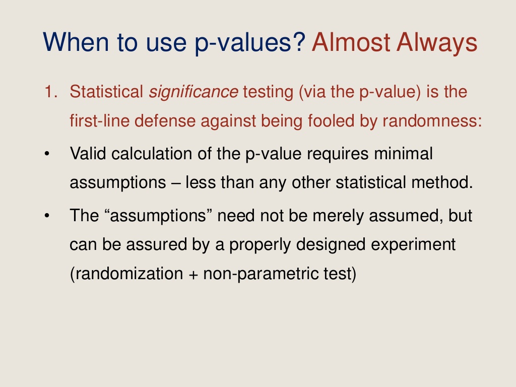
.
These were Yoav Benjamini’s slides,”In the world beyond p<.05: When & How to use P<.0499…” from our session at the ASA 2017 Symposium on Statistical Inference (SSI): A World Beyond p < 0.05. (Mine are in an earlier post.) He begins by asking:
.
There will be a roundtable on reproducibility Friday, October 27th (noon Eastern time), hosted by the International Methods Colloquium, on the reproducibility crisis in social sciences motivated by the paper, “Redefine statistical significance.” Recall, that was the paper written by a megateam of researchers as part of the movement to require p ≤ .005, based on appraising significance tests by a Bayes Factor analysis, with prior probabilities on a point null and a given alternative. It seems to me that if you’re prepared to scrutinize your frequentist (error statistical) method on grounds of Bayes Factors, then you must endorse using Bayes Factors (BFs) for inference to begin with. If you don’t endorse BFs–and, in particular, the BF required to get the disagreement with p-values–*, then it doesn’t make sense to appraise your non-Bayesian method on grounds of agreeing or disagreeing with BFs. For suppose you assess the recommended BFs from the perspective of an error statistical account–that is, one that checks how frequently the method would uncover or avoid the relevant mistaken inference.[i] Then, if you reach the stipulated BF level against a null hypothesis, you will find the situation is reversed, and the recommended BF exaggerates the evidence! (In particular, with high probability, it gives an alternative H’ fairly high posterior probability, or comparatively higher probability, even though H’ is false.) Failing to reach the BF cut-off, by contrast, can find no evidence against, and even finds evidence for, a null hypothesis with high probability, even when non-trivial discrepancies exist. They’re measuring very different things, and it’s illicit to expect an agreement on numbers.[ii] We’ve discussed this quite a lot on this blog (2 are linked below [iii]).
If the given list of panelists is correct, it looks to be 4 against 1, but I’ve no doubt that Lakens can handle it.

Over 100 patients signed up for the chance to participate in the clinical trials at Duke (2007-10) that promised a custom-tailored cancer treatment spewed out by a cutting-edge prediction model developed by Anil Potti, Joseph Nevins and their team at Duke. Their model purported to predict your probable response to one or another chemotherapy based on microarray analyses of various tumors. While they are now described as “false pioneers” of personalized cancer treatments, it’s not clear what has been learned from the fireworks surrounding the Potti episode overall. Most of the popular focus has been on glaring typographical and data processing errors—at least that’s what I mainly heard about until recently. Although they were quite crucial to the science in this case,(surely more so than Potti’s CV padding) what interests me now are the general methodological and logical concerns that rarely make it into the popular press. Continue reading
We are pleased to announce our guest speaker at Thursday’s seminar (April 24, 2014): “Statistics and Scientific Integrity”:
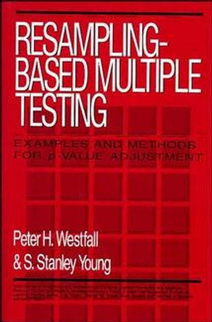
 S. Stanley Young, PhD
Assistant Director for Bioinformatics
National Institute of Statistical Sciences
Research Triangle Park, NC
Author of Resampling-Based Multiple Testing, Westfall and Young (1993) Wiley.
The main readings for the discussion are:
 Below are slides from March 6, 2014: (a) the 2nd half of “Frequentist Statistics as a Theory of Inductive Inference” (Selection Effects),”* and (b) the discussion of the Higgs particle discovery and controversy over 5 sigma.
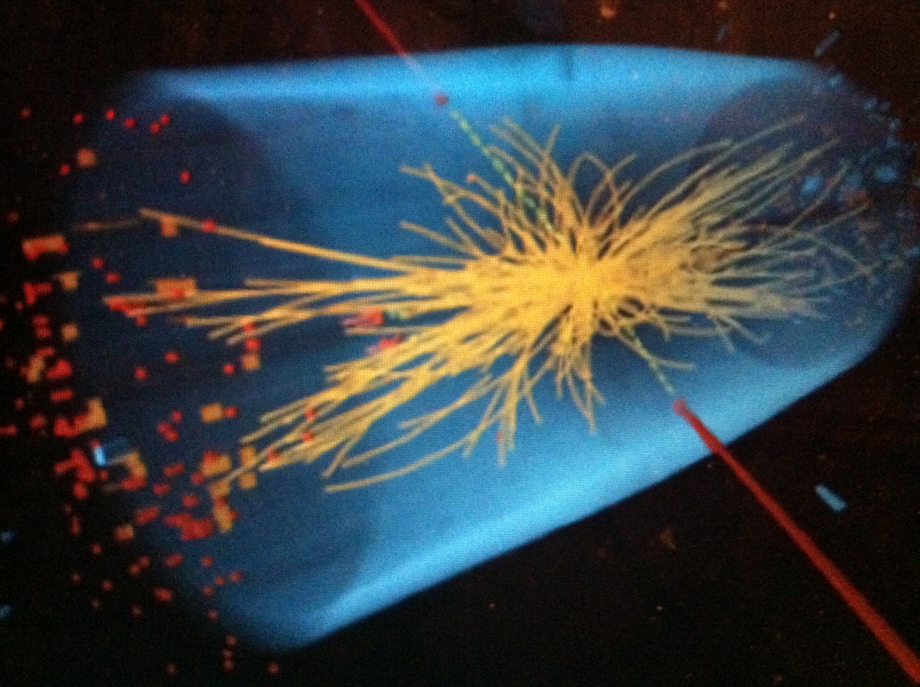
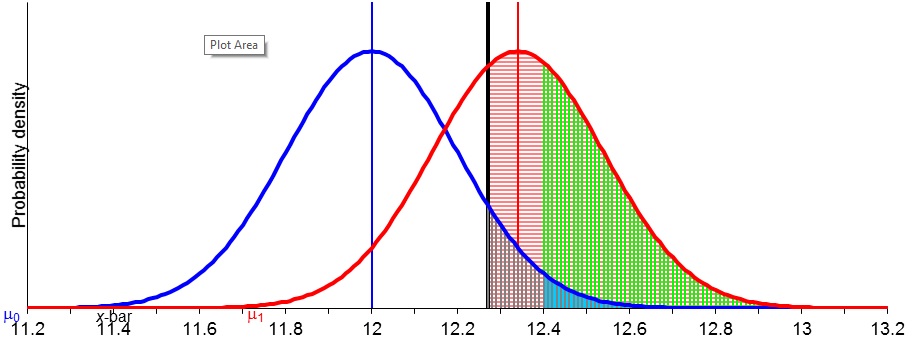
We spent the rest of the seminar computing significance levels, rejection regions, and power (by hand and with the Excel program). Here is the updated syllabus (3rd installment).
A relevant paper on selection effects on this blog is here.

DGM playing the slots
I may have been exaggerating one year ago when I started this post with “Hardly a day goes by”, but now it is literally the case*. (This also pertains to reading for Phil6334 for Thurs. March 6):
Hardly a day goes by where I do not come across an article on the problems for statistical inference based on fallaciously capitalizing on chance: high-powered computer searches and “big” data trolling offer rich hunting grounds out of which apparently impressive results may be “cherry-picked”:
When the hypotheses are tested on the same data that suggested them and when tests of significance are based on such data, then a spurious impression of validity may result. The computed level of significance may have almost no relation to the true level. . . . Suppose that twenty sets of differences have been examined, that one difference seems large enough to test and that this difference turns out to be “significant at the 5 percent level.” Does this mean that differences as large as the one tested would occur by chance only 5 percent of the time when the true difference is zero? The answer is no, because the difference tested has been selected from the twenty differences that were examined. The actual level of significance is not 5 percent, but 64 percent! (Selvin 1970, 104)[1]
…Oh wait -this is from a contributor to Morrison and Henkel way back in 1970! But there is one big contrast, I find, that makes current day reports so much more worrisome: critics of the Morrison and Henkel ilk clearly report that to ignore a variety of “selection effects” results in a fallacious computation of the actual significance level associated with a given inference; clear terminology is used to distinguish the “computed” or “nominal” significance level on the one hand, and the actual or warranted significance level on the other. Continue reading
 Stephen Senn
Head, Methodology and Statistics Group,
Competence Center for Methodology and Statistics (CCMS),
Luxembourg
“Dawid’s Selection Paradox”
You can protest, of course, that Dawid’s Selection Paradox is no such thing but then those who believe in the inexorable triumph of logic will deny that anything is a paradox. In a challenging paper published nearly 20 years ago (Dawid 1994), Philip Dawid drew attention to a ‘paradox’ of Bayesian inference. To describe it, I can do no better than to cite the abstract of the paper, which is available from Project Euclid, here: http://projecteuclid.org/DPubS/Repository/1.0/Disseminate?
When the inference to be made is selected after looking at the data, the classical statistical approach demands — as seems intuitively sensible — that allowance be made for the bias thus introduced. From a Bayesian viewpoint, however, no such adjustment is required, even when the Bayesian inference closely mimics the unadjusted classical one. In this paper we examine more closely this seeming inadequacy of the Bayesian approach. In particular, it is argued that conjugate priors for multivariate problems typically embody an unreasonable determinism property, at variance with the above intuition.
I consider this to be an important paper not only for Bayesians but also for frequentists, yet it has only been cited 14 times as of 15 November 2013 according to Google Scholar. In fact I wrote a paper about it in the American Statistician a few years back (Senn 2008) and have also referred to it in a previous blogpost (12 May 2012). That I think it is important and neglected is excuse enough to write about it again.
Philip Dawid is not responsible for my interpretation of his paradox but the way that I understand it can be explained by considering what it means to have a prior distribution. First, as a reminder, if you are going to be 100% Bayesian, which is to say that all of what you will do by way of inference will be to turn a prior into a posterior distribution using the likelihood and the operation of Bayes theorem, then your prior distribution has to satisfy two conditions. First, it must be what you would use to bet now (that is to say at the moment it is established) and second no amount of subsequent data will change your prior qua prior. It will, of course, be updated by Bayes theorem to form a posterior distribution once further data are obtained but that is another matter. The relevant time here is your observation time not the time when the data were collected, so that data that were available in principle but only came to your attention after you established your prior distribution count as further data.
Now suppose that you are going to make an inference about a population mean, θ, using a random sample from the population and choose the standard conjugate prior distribution. Then in that case you will use a Normal distribution with known (to you) parameters μ and σ2. If σ2 is large compared to the random variation you might expect for the means in your sample, then the prior distribution is fairly uninformative and if it is small then fairly informative but being uninformative is not in itself a virtue. Being not informative enough runs the risk that your prior distribution is not one you might wish to use to bet now and being too informative that your prior distribution is one you might be tempted to change given further information. In either of these two cases your prior distribution will be wrong. Thus the task is to be neither too informative nor not informative enough. Continue reading

")

Experts convene to explore new philosophy of statistics field

