

.
Stephen Senn
Consultant Statistician
Edinburgh
What is this n you boast about?
Failure to understand components of variation is the source of much mischief. It can lead researchers to overlook that they can be rich in data-points but poor in information. The important thing is always to understand what varies in the data you have, and to what extent your design, and the purpose you have in mind, master it. The result of failing to understand this can be that you mistakenly calculate standard errors of your estimates that are too small because you divide the variance by an n that is too big. In fact, the problems can go further than this, since you may even pick up the wrong covariance and hence use inappropriate regression coefficients to adjust your estimates.
I shall illustrate this point using clinical trials in asthma.
Breathing lessons
Suppose that I design a clinical trial in asthma as follows. I have six centres, each centre has four patients, each patient will be studied in two episodes of seven days and during these seven days the patients will be measured daily, that is to say, seven times per episode. I assume that between the two episodes of treatment there is a period of some days in which no measurements are taken. In the context of a cross-over trial, which I may or may not decide to run, such a period is referred to as a washout period.
The block structure is like this:
Centres/Patients/Episodes/Measurements
The / sign is a nesting operator and it shows, for example, that I have Patients ‘nested’ within centres. For example, I could label the patients 1 to 4 in each centre, but I don’t regard patient 3 (say) in centre 1 as being somehow similar to patient 3 in centre 2 and patient 3 in centre 3 and so forth. Patient is a term that is given meaning by referring it to centre.
The block structure is shown in Figure 1, which does not, however, show the seven measurements per episode.
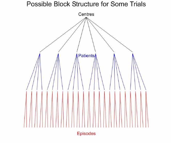
Figure 1. Schematic representation of the block structure for some possible clinical trials. The six centres are shown by black lines. For each centre there are four patients shown by blue lines and each patient is studied in two episodes, shown by red lines.
I now wish to compare two treatments, two so-called beta-agonists. The first of these, I shall call Zephyr and the second Mistral. I shall do this using a measure of lung function called forced expiratory volume in one second, (FEV1). If there are no dropouts and no missing measurements, I shall have 6 x 4 x 2 x 7 =336 FEV1 readings. Is this my ‘n’?
I am going to use Genstat®, a package that fully incorporates John Nelder’s ideas of general balance[1, 2]and the analysis of designed experiments and uses, in fact, what I have called the Rothamsted approach to experiments.
I start by declaring the block structure thus
BLOCKSTRUCTURE Centre/Patient/Episode/Measurement
This is the ‘null’ situation: it describes the variation in the experimental material before any treatment is applied. If I ask Genstat®to do a ‘null’ skeleton analysis of variance for me, by typing the statement
ANOVA
and the output is as given in Table 1
Analysis of variance
| Source of variation | d.f. |
| Centre stratum | 5 |
| Centre.Patient stratum | 18 |
| Centre.Patient.Episode stratum | 24 |
| Centre.Patient.Episode.Measurement stratum | 288 |
| Total | 335 |
Table 1. Degrees of freedom for a null analysis of variance for a nested block structure.
This only gives me possible sources of variation and degrees of freedom associated with them but not the actual variances: that would require data. There are six centres, so five degrees of freedom between centres. There are four patients per centre, so three degrees of freedom per centre between patients but there are six centres and therefore 6 x 3 = 18 in total. There are two episodes per patient and so one degree of freedom between episodes per patient but there are 24 patients and so 24 degrees of freedom in total. Finally, there are seven measurements per episode and hence six degrees of freedom but 48 episodes in total so 48 x 6 = 288 degrees of freedom for measurements.
Having some actual data would put flesh on the bones of this skeleton by giving me some mean square errors, but to understand the general structure this is not necessary. It tells me that at the highest level I will have variation between centres, next patients within centres, after that episodes within patients and finally measurements within episodes. Which of these are relevant to judging the effect of any treatments I wish to study depends how I allocate treatments.
Design matters
I now consider, three possible approaches to allocating treatments to patients. In each of the three designs, the same number of measurements will be available for each treatment. There will be 168 measurements under Zephyr and 168 measurements under Mistral and thus 336 in total. However, as I shall show, the designs will be very different, and this will lead to different analyses being appropriate and lead us to understand better what our n is.
I shall also suppose that we are interested in causal analysis rather than prediction. That is to say, we are interested in estimating the effect that the treatments did have (actually, the difference in their effects) in the trial that was actually run. The matter of predicting what would happen in future to other patients is much more delicate and raises other issues and I shall not address it here, although I may do so in future. For further discussion see my paper Added Values[3].
In the first experiment, I carry out a so-called cluster-randomised trial. I choose three centres at random and all patents, in both episodes on all occasions in the three centres chosen receive Zephyr. For the other three centres, all patients on all occasions receive Mistral. I create a factor Treatment (cluster trial), (Cluster for short) which encodes this allocation so that the pattern of allocation to Zephyr or Mistral reflects this randomised scheme.
In the second experiment, I carry out a parallel group trial blocking by centre. In each centre, I choose two patients to receive Zephyr and two to receive Mistral. Thus, overall, there 6 x 2 = 12 patients on each treatment. I create a factor Treatment (parallel trial) (Parallel for short) to reflect this.
The third experiment consists of a cross-over trial. Each patient is randomised to one of two sequences, either receiving Zephyr in episode one and Mistral in episode two, or vice versa. Each patient receives both treatments so that there will be 6 x 4 = 24 patients given each treatment. I create a factor Treatment (cross-over trial) (Cross-over for short) to encode this.
Note that the total number of measurements obtained is the same for each of the three schemes. For the cluster randomised trial, a given treatment will be studied in three centres each of which has four patients, each of whom will be studied in two episodes on seven occasions. Thus, we have 3 x 4 x 2 x 7 = 168 measurement per treatment. For the parallel group trial, 12 patients are studied for a given treatment in two episodes, each providing 7 measurements. Thus, we have 12 x 2 x 7 = 168 measurement per treatment. For the cross-over trial we have 24 patients each of whom will receive a given treatment in one episode (either episode one or two) so we have 24 x 1 x 7 + 168 measurements per treatment.
Thus, from one point of view the n in the data is the same for each of these three designs. However, each of the three designs provides very different amounts of information and this alone should be enough to warn anybody against assuming that all problems of precision can be solved by increasing the number of data.
Controlled Analysis
Before collecting any data, I can analyse this scheme and use Nelder’s approach to tell me where the information is in each scheme.
Using the three factors to encode the corresponding allocation, I now ask Genstat® to prepare a dummy analysis of variance (in advance of having collected any data) as follows. All I need to do is type a statement of the form
TREATMENTSTRUCTURE Design
ANOVA
Where Design is set equal to the Cluster, Parallel, Crossover, as the case may be. The result is shown in Table 2
Analysis of variance
| Source of variation | d.f. |
| Centre stratum | |
| Treatment (cluster trial) | 1 |
| Residual | 4 |
| Centre.Patient stratum | |
| Treatment (parallel trial) | 1 |
| Residual | 17 |
| Centre.Patient.Episode stratum | |
| Treatment (cross-over trial) | 1 |
| Residual | 23 |
| Centre.Patient.Episode.Measurement stratum | 288 |
| Total | 335 |
Table 2. Analysis of variance skeleton for three possible designs using the block structure given in Table 1
This shows us that the three possible designs will have quite different degrees of precision associated with them. Since, for the cluster trial, any given centre only receives one of the treatments, the variation between centres affects the estimate of the treatment effect and its standard error must reflect this. Since, however, the parallel trial balances treatments by centres it is unaffected by variation between centres. It is, however, affected by variation between patients. This variation is, in turn, eliminated by the cross-over trial which, in consequence is only affected by variation between episodes (although this variation will, itself, inherit variation from measurements). Each higher level of variation inherits variation from the lower levels but adds its own.
Note, however, that for all three designs the unbiased estimate of the treatment effect is the same. All that is necessary is to average the 168 measurements under Zephyr and the 168 under Mistral and calculate the difference. It is the estimate of the appropriate variation in the estimate that varies.
Suppose that, more generally, we have m centres, with n patients per centre and p episodes per patient, with the number of measurements per episode fixed, then for the cross-over trial the variance of our estimate will be proportional to 


The consequences of this are, you cannot decrease the variance of a cluster randomised trial indefinitely simply by increasing the number of patients; it is centres you need to increase. You cannot decrease the variance of a parallel group trial indefinitely by increasing the number of episodes; it is patients you need to increase.
Degrees of Uncertainty
Why should this matter? Why should it matter how certain we are about anything? There are several reasons. Bayesian statisticians need to know what relative weight to give their prior belief and the evidence from the data. If they do not, they do not know how to produce a posterior distribution. If they do not know what the variances of both data and prior are, they don’t know the posterior variance. Frequentists and Bayesians are often required to combine evidence from various sources as, say, in a so-called meta-analysis. They need to know what weight to give to each and again to assess the total information available at the end. Any rational approach to decision-making requires an appreciation of the value of information. If one had to make a decision with no further prospect of obtaining information based on a current estimate it might make little difference how precise it was but if the option of obtaining further information at some cost applies, this is no longer true. In short, estimation of uncertainty is important. Indeed, it is a central task of statistics.
Finally, there is one further point that is important. What applies to variances also applies to covariances. If you are adjusting for a covariate using a regression approach, then the standard estimate of the coefficient of adjustment will involve a covariance divided by a variance. Just as there can be variances at various levels there can be covariances at various levels. It is important to establish which is relevant[4] otherwise you will calculate the adjustment incorrectly.
Consequences
Just because you have many data does not mean that you will come to precise conclusions: the variance of the effect estimate may not, as one might naively suppose, be inversely proportional to the number of data, but to some other much rarer feature in the data-set. Failure to appreciate this has led to excessive enthusiasm for the use of synthetic patients and historical controls as alternatives to concurrent controls. However, the relevant dominating component of variation is that between studies not between patients. This does not shrink to zero as the number of subjects goes to infinity. it does not even shrink to zero as the number of studies goes to infinity, since if the current study is the only one that the new treatment is on, the relevant variance for that arm is at least 
There is a lesson also for epidemiology here. All too often, the argument in the epidemiological, and more recently, the causal literature has been about which effects one should control for or condition on without appreciating that merely stating what should be controlled for does not solve how. I am not talking here about the largely sterile debate, to which I have contributed myself[5] as to how at a given level, adjustment should be made for possible confounders (for example, propensity score or linear model), but to the level at which such adjustment can be made. The usual implicit assumption is that an observational study is somehow a deficient parallel group trial, with maybe complex and perverse allocation mechanisms that must somehow be adjusted for, but that once such adjustments have been made, precision increases as the subjects increase. But suppose the true analogy is a cluster randomised trial. Then, whatever you adjust for, your standard errors will be too small.
Finally, it is my opinion, that much of the discussion about Lord’s paradox would have benefitted from an appreciation of the issue of components of variance. I am used to informing medical clients that saying we will analyse the data using analysis of variance is about as useful as saying we will treat the patients with a pill. The varieties of analysis of variance are legion and the same is true of analysis of covariance. So, you conditioned on the baseline values. Bravo! But how did you condition on them? If you used a slope obtained at the wrong level of the data then, except fortuitously, your adjustment will be wrong, as will the precision you claim for it.
Finally, if I may be permitted an auto-quote, the price one pays for not using concurrent control is complex and unconvincing mathematics. That complexity may be being underestimated by those touting ‘big data’.
.
References
- Nelder JA. The analysis of randomised experiments with orthogonal block structure I. Block structure and the null analysis of variance. Proceedings of the Royal Society of London. Series A 1965; 283: 147-162.
- Nelder JA. The analysis of randomised experiments with orthogonal block structure II. Treatment structure and the general analysis of variance. Proceedings of the Royal Society of London. Series A 1965; 283: 163-178.
- Senn SJ. Added Values: Controversies concerning randomization and additivity in clinical trials. Statistics in Medicine 2004; 23: 3729-3753.
- Kenward MG, Roger JH. The use of baseline covariates in crossover studies. Biostatistics2010; 11: 1-17.
- Senn SJ, Graf E, Caputo A. Stratification for the propensity score compared with linear regression techniques to assess the effect of treatment or exposure. Statistics in Medicine 2007; 26: 5529-5544.
Some relevant blogposts
Lord’s Paradox:
Personalized Medicine:
-
- (01/30/18) S. Senn: Evidence Based or Person-centred? A Statistical debate (Guest Post)
- (7/11/18) S. Senn: Personal perils: are numbers needed to treat misleading us as to the scope for personalised medicine? (Guest Post)
- (07/26/14) S. Senn: “Responder despondency: myths of personalized medicine” (Guest Post)
Randomisation:
-
- (07/01/17) S. Senn: Fishing for fakes with Fisher (Guest Post)


")


Would you agree that informative priors are needed for the between study variances you mention when there are few studies or even only one?
Keith O’Rourke
Yes. Variance components are a delicate thing to estimate and you usually need a reasonable number of degrees of freedom. However, I was describing orthogonal designs. If you have the same number of patients per cluster and the same number of observations per patient the information only needs to be estimated at the highest level so the issue of weighting of information at different levels does not arise. Nevertheless, you still need some degrees of freedom. In fact, in my previous posts on Lord Paradox, I pointed out that it was failure to appreciate this that led to the confusion I identified in the Book of Why.
I’m very grateful to Stephen Senn for this guest post! Thank you Stephen.
You are very welcome. I am grateful to have it hosted!
Pingback: A talk by Stephen Senn | Peter Cameron's Blog
Stephen,
Your exposition of how one’s n may be “too big” and lead to what in many disciplines since 1984 has been termed “pseudoreplication” (1) may be satisfactory for some professional statisticians but for many other scientists, it would benefit from use of the core and classical, if much neglected, terminology of experimental design (1,2)., e.g. experimental unit, evaluation unit, block, treatment structure, design (or error control) structure, response structure. Most statistics texts either do not define these at all or misdefine or mischaracterize them. The majority of statisticians (and the people they advise) post-Cox’s 1958 Planning of Experiments, is pretty much AWOL on the matter. Many are to blame, but it was primarily the psychologists who initiated the disorderly retreat from the classical terminology developed by your friends and their predecessors at Harpenden. Delicate, unimaginative souls, the psychologists couldn’t relate to examples using “plots” and “manure treatments”.
Statisticians and others who misjudge the “size of their n” do not understand the simple concept of the experimental unit. The various types of pseudoreplication (simple, temporal, sacrificial & their combinations) all reflect confusion about the difference between experimental units and evaluation units. For a few decades I taught Experimental Design to biology students with only 1-2 prior semesters of statistics, and each had to critique the designs and analyses in 25 published papers and tabulate errors found. As a quick check on the presence of pseudoreplication, I told them to look at the methods section and determine the number of treatments (a) and the number of experimental units per treatment (n), and then to look at the Results section and make sure the error d.f. for the test for a treatment effect were less than or equal to a(n-1). If it was greater, they had to “reel it in” for a more detailed diagnosis (post mortem?) on deck, and almost always found a bad case of pseudoreplication and additional problems as well. In some paper sets it was found in more than 30-60% of the papers, and big name biologists and statisticians were on plenty of these. Error d.f. used in a paper were sometimes 1-2 orders of magnitude greater than allowed by the actual design. Quite empowering for the students who then occasionally got into hot water by pointing out the problem in papers by their thesis or dissertation adviser.
Hurlbert, S.H. 2009. The ancient black art and transdisciplinary extent of pseudoreplication. Journal of Comparative Psychology 123: 434-443.
Hurlbert, S.H. 2013. Affirmation of the classical terminology for experimental design via a critique of Casella’s Statistical Design. Agronomy Journal 105: 412-418 + suppl. inform.
I agree with Stuart Hurlbert that this may not make easy reading but he perhaps missed that this was one of three linked posts on the subject of block structure, the other two being https://errorstatistics.com/2018/11/11/stephen-senn-rothamsted-statistics-meets-lords-paradox-guest-post/ and https://errorstatistics.com/2018/11/22/stephen-senn-on-the-level-why-block-structure-matters-and-its-relevance-to-lords-paradox-guest-post/ , both of which made extensive use of blocks as a concept. Nevertheless, judging by the response from the causal modelling world, the message was not understood, so maybe further explanation, such as he provides, will help. We shall see. Judging by the responses, causal modelling does not appear to distinguish between a diet that is varied between halls and one that is varied at the level of students within halls. I take it that Stuart agrees with me that this is a fundamental distinction.
To pick up the theme of modelling and pseudo-replication, I think that one of the problems is that superficial structural similarities in measurement are mistaken (or perhaps substituted for) for fundamental ones in terms of allocation. One of my personal bugbears is that data-sets involving repeated measures are analysed using the so-called split-plot approach despite the fact that no randomisation is possible at that level, time being, notoriously, like all history, a case of ‘one damn thing after another’. See Yates, F., Reader Reaction – Regression-Models for Repeated Measurements. Biometrics, 1982. 38(3): p. 850-853. for a trenchant criticism.
I think that the degrees of freedom exercise which Stuart stresses is very useful (and i shall certainly check the references). However, one of the issues is that here it is not just the design but also the purpose (purely causal analysis as to what happened or predictive analysis as to what might happen) that affects the choice of error variance. See
Senn, S.J., Added Values: Controversies concerning randomization and additivity in clinical trials. Statistics in Medicine, 2004. 23(24): p. 3729-3753.for some discussion
and
Araujo, A., S. Julious, and S. Senn, Understanding Variation in Sets of N-of-1 Trials. PLOS ONE, 2016. 11(12): p. e0167167.
for an application.
Stephen,
I won’t say anything about causal modeling here on the principle it’s best to keep silent on matters where one is totally ignorant of the literature (and w/o time to remedy the situation).
I too have long had a “bugbear” on the longstanding terminological sloppiness where split-unit design structures are confused with repeated measures response structures (or sometimes even with the use of multiple response variables). A lot of the confusion can be traced to Cornellians (Federer, Steel & Torrie, Casella). If you’d like a more recent and extended discussion of the issue than Yates (1982), there is one in “Affirmation of the classical terminology” that I cited earlier. And even longer one is given in pp. 654-657 of :
Hurlbert, S.H. 2012. Pseudofactorialism, response structures, and collective responsibility. Austral Ecology 38: 646-663 + suppl. inform. (will send you a pdf).
Stuart
Pingback: S. Senn: “Error point: The importance of knowing how much you don’t know” (guest post) | Error Statistics Philosophy