

.
We’re going to be discussing the philosophy of m-s testing today in our seminar, so I’m reblogging this from Feb. 2012. I’ve linked the 3 follow-ups below. Check the original posts for some good discussion. (Note visitor*)
“This is the kind of cure that kills the patient!”
is the line of Aris Spanos that I most remember from when I first heard him talk about testing assumptions of, and respecifying, statistical models in 1999. (The patient, of course, is the statistical model.) On finishing my book, EGEK 1996, I had been keen to fill its central gaps one of which was fleshing out a crucial piece of the error-statistical framework of learning from error: How to validate the assumptions of statistical models. But the whole problem turned out to be far more philosophically—not to mention technically—challenging than I imagined. I will try (in 3 short posts) to sketch a procedure that I think puts the entire process of model validation on a sound logical footing. Thanks to attending several of Spanos’ seminars (and his patient tutorials, for which I am very grateful), I was eventually able to reflect philosophically on aspects of his already well-worked out approach. (Synergies with the error statistical philosophy, of which this is a part, warrant a separate discussion.)
Problems of Validation in the Linear Regression Model (LRM)
The example Spanos was considering was the the Linear Regression Model (LRM) which may be seen to take the form:
M0: yt = β0 + β1xt + ut, t=1,2,…,n,…
Where µt = β0 + β1xt is viewed as the systematic component, and ut = yt – β0 – β1xt as the error (non-systematic) component. The error process {ut, t=1, 2, …, n, …,} is assumed to be Normal, Independent and Identically Distributed (NIID) with mean 0, variance σ2 , i.e. Normal white noise. Using the data z0:={(xt, yt), t=1, 2, …, n} the coefficients (β0 , β1) are estimated (by least squares)yielding an empirical equation intended to enable us to understand how yt varies with Xt.
Empirical Example
Suppose that in her attempt to find a way to understand and predict changes in the U.S.A. population, an economist discovers, using regression, an empirical relationship that appears to provide almost a ‘law-like’ fit (see figure 1):
yt = 167.115+ 1.907xt + ût, (1)
where yt denotes the population of the USA (in millions), and xt denotes a secret variable whose identity is not revealed until the end (these 3 posts). Both series refer to annual data for the period 1955-1989.
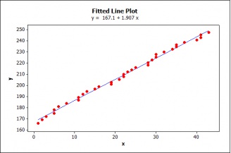
Figure 1: Fitted Line
A Primary Statistical Question: How good a predictor is xt?
The goodness of fit measure of this estimated regression, R2=.995, indicates an almost perfect fit. Testing the statistical significance of the coefficients shows them to be highly significant, p-values are zero (0) to a third decimal, indicating a very strong relationship between the variables. Everything looks hunky dory; what could go wrong?
Is this inference reliable? Not unless the data z0 satisfy the probabilistic assumptions of the LRM, i.e., the errors are NIID with mean 0, variance σ2.
Misspecification (M-S) Tests: Questions of model validation may be seen as ‘secondary’ questions in relation to primary statistical ones; the latter often concern the sign and magnitude of the coefficients of this linear relationship.
Partitioning the Space of Possible Models: Probabilistic Reduction (PR)
The task in validating a model M0 (LRM) is to test ‘M0is valid’ against everything else!
In other words, if we let H0 assert that the ‘true’ distribution of the sample Z, f(z) belongs to M0, the alternative H1 would be the entire complement of M0, more formally:
H0: f(z) € M0 vs. H1: f(z) € [P – M0]
where P denotes the set of all possible statistical models that could have given rise to z0:={(xt,yt), t=1, 2, …, n}, and € is “an element of” (all we could find).
The traditional analysis of the LRM has already, implicitly, reduced the space of models that could be considered. It reflects just one way of reducing the set of all possible models of which data z0 can be seen to be a realization. This provides the motivation for Spanos’ modeling approach (first in Spanos 1986, 1989, 1995).
Given that each statistical model arises as a parameterization from the joint distribution:
D(Z1,…,Zn;φ): = D((X1, Y1), (X2, Y2), …., (Xn, Yn); φ),
we can consider how one or another set of probabilistic assumptions on the joint distribution gives rise to different models. The assumptions used to reduce P, the set of all possible models, to a single model, here the LRM, come from a menu of three broad categories. These three categories can always be used in statistical modeling:
(D) Distribution, (M) Dependence, (H) Heterogeneity.
For example, the LRM arises when we reduce P by means of the “reduction” assumptions:
(D) Normal (N), (M) Independent (I), (H) Identically Distributed (ID).
Since we are partitioning or reducing P by means of the probabilistic assumptions, it may be called the Probabilistic Partitioning or Probabilistic Reduction (PR) approach.[i]
The same assumptions, traditionally given by means of the error term, are instead specified in terms of the observable random variables (yt, Xt): [1]-[5] in table 1 to render them directly assessable by the data in question.
| Table 1 – The Linear Regression Model (LRM) | ||
|
yt = β0 + β1xt + ut, t=1,2,…,n,… |
||
| [1] Normality: | D(yt |xt; θ) | Normal |
| [2] Linearity: | E(yt |Xt=xt) = β0 + β1xt | Linear in xt |
| [3] Homoskedasticity: | Var(yt |Xt=xt) =σ2, | Free of xt |
| [4] Independence: | {(yt |Xt=xt), t=1,…,n,…} | Independent |
| [5] t-invariance: | θ:=(β0 , β1, σ2), | constant over t |
There are several advantages to specifying the model assumptions in terms of the observables yt and xt instead of the unobservable error term.
First, hidden or implicit assumptions now become explicit ([5]).
Second, some of the error term assumptions, such as having a zero mean, do not look nearly as innocuous when expressed as an assumption concerning the linearity of the regression function between yt and xt .
Third, the LRM (conditional) assumptions can be assessed indirectly from the data via the (unconditional) reduction assumptions, since:
N entails [1]-[3], I entails [4], ID entails [5].
As a first step, we partition the set of all possible models coarsely
in terms of reduction assumptions on D(Z1,…,Zn;φ):
| LRM | Alternatives | |
| (D) Distribution: | Normal | non-Normal |
| (M) Dependence: | Independent | Dependent |
| (H) Heterogeneity: | Identically Distributed | Non-ID |
Given the practical impossibility of probing for violations in all possible directions, the PR approach consciously considers an effective probing strategy to home in on the directions in which the primary statistical model might be potentially misspecified. Having taken us back to the joint distribution, why not get ideas by looking at yt and xt themselves using a variety of graphical techniques? This is what the Probabilistic Reduction (PR) approach prescribes for its diagnostic task….Stay tuned!
*Rather than list scads of references, I direct the interested reader to those in Spanos.
[i] This is because when the NIID assumptions are imposed on the latter simplifies into a product of conditional distributions (LRM).
See follow-up parts:
PART 2: https://errorstatistics.com/2012/02/23/misspecification-testing-part-2/
PART 3: https://errorstatistics.com/2012/02/27/misspecification-testing-part-3-m-s-blog/
PART 4: https://errorstatistics.com/2012/02/28/m-s-tests-part-4-the-end-of-the-story-and-some-conclusions/
*We also have a visitor to the seminar from Hawaii, John Byrd, a forensic anthropologist and statistical osteometrician. He’s long been active on the blog. I’ll post something of his later on.


")


I have a couple of comments.
First the independence assumption is very important but in many contexts it is not a question of diagnostics alone. Statisticians can, and frequently do, analyse randomised clinical trials using linear models. In a parallel group trial you might assume independence of disturbance terms (OK, Aris wants us to stop thinking in terms of disturbance terms) but in other sorts of trials (for example cluster randomised) you would not, and for yet others (for example cross-over trials) the modelling would be at the level of treatment episodes and you would not assume independence of episodes. In these sorts of contexts, independence is an assumption made conditionally at some level as a consequence of the design and background knowledge. It is not a matter of diagnostics.
Second, in using any diagnostic approach one has to be careful. Medicine shows us why. What could be harmful about screening patients for disease? (At least if the screening is free and non-invasive.) Nothing, surely, since more information is always better than less. However, in practice, it turns out that doctors tend to make inappropriate decisions what to do next based on the evidence from a screen. To provide reassurance that screening is a good thing the joint strategy screening + therapy needs to be studied. A similar point is necessary for model diagnostics. As long ago as 1944 Bancroft published a paper ‘On biases in estimation due to use of preliminary tests of significance Ann. Math Statist, 15, 190-204 that showed there could be a problem.
Stephen: Thanks for the comment. It may make a difference that Aris is working in the context of non-experimental data. Also, I think the concern about pre-testing biases, or however you’d describe your last remark, is one he’d dismiss, at least for the subsequent steps he would recommend. It’s interesting that you compare it to medical diagnostics though.
In this connection, if I hear an article or doctor telling me that on average in the long run I won’t live longer if I get this diagnostic test, I think their computations are irrelevant for what I want to know.
Deborah: The pre-testing issue is a serious one. The same data are used twice. I thought this was something the error-statistics school was concerned about. You can see that I raised this as an issue in commenting on Gelman and Shalizi. I don’t see why I should give Spanos a free ride.
As for your screening point, I consider that it is the overall result that matters.(I am not sure from your comment whether you do or don’t.) In decision-making average risks are relevant except to the extent that you can recongise relevant subsets. What needs to be recognised is that this applies to statistics as well as medicine.
A final point: Deming pointed out that managers who did not study and understand the performance of the system as a whole tended to intervene in ways that seemed good but in practice harmed quality. This is potentially a harm to modelling also. Thus I require to know how the overall 1. process diagnostics + 2. model choice + 3. analysis using final model works.
Stephen: It depends what the system as a whole amounts to, and whether one is viewing the scientific output as a behavioristic or evidential one. Following Cox, the joint paper Mayo and Cox (2006/10) listed the secondary model checking case as not altering error probabilities for the primary inference. Other contexts may differ.
In addition to Stephen’s comments;
It’s not, in general, enough to start off with the premise that one wants to “understand and predict” something.
If by “understand”, you making causal inferences, you need more assumptions than purely statistical ones. Assessing these assumptions is futile without knowing what x is, so the didactic device of keeping it “secret” is not helpful. Why might differences in mean Y at different levels of x plausibly tell us about some causal relationship? What confounding factors might be at play? Thinking hard about these is often vastly more important than whether Normality and linearity hold. Dependence is arguably different, as confounding factors might lead to the dependence, but even this is not automatic. (And if you don’t mean to give causal inference, what do you mean?)
The statistical meaning of “predict” is less ambiguous; we want to do the best possible job of predicting new observations. Without going into the guts of all the statistical tools one can use for that job, it should be noted that they are *different* to those used for causal inference, i.e. “understanding”, and the extent to which Normality, linearity etc are crucial to their output may also differ.
So, one might want to understand OR predict the population of the USA based on some X, but one’s concerns about mis-specification can vary depending on which task we’re doing, and may depend very much on what that X actually is.
OG: I take it that, in a sense, this is precisely the lesson of the exercise with the unknown x (so much a part of big data/ black box enterprises). It all looks swell from the familiar statistical perspective. Nothing in this approach ignores underlying theory or causal knowledge, but on the way toward arriving at that knowledge, it’s valuable to find ways to extract more information from statistical probing.It’s an iterative procedure.
No, it doesn’t “all look swell” from the statistical perspective, because you’ve given no real indication of what the statistical analysis is for, nor have you said how the data were obtained, nor even given a complete picture of what the variables are. Statisticians go to considerable efforts to understand such issues, before modeling begins.
Concern over model mis-specification without first making such efforts is like worrying over the arrangement of the Titanic’s deckchairs.
OG: Nothing in what was said ignores how the data were obtained nor what the known variables are, there was a very specific purpose in the illustration. I don’t know where you get the Titanic’s deckchain allegation. This technique grows out of a general to specific perspective with the variables stemming from theory.Please give us your recommended way to testing statistical model assumptions at whatever stage you think appropriate. I did say this was non-experimental.
“Nothing in what was said ignores how the data were obtained nor what the known variables are”
Yes it does, you haven’t said how X was sampled each year, nor what X actually represents. And you still haven’t stated the purpose of the analysis, to which one should be tailoring any diagnostics.
My recommendations start out by saying what the analysis is for, what the data is, and where the data came from.
OG: I was referring to the general program for m-s testing. It was part of this little exercise to imagine X as a mystery, it’s not part of the account.
Stephen: Many thanks for the Bancroft reference. This is great. I wasn’t aware of this, although I’m interested for a long time in this kind of considerations. (I know that a few things have been done much later.)
General: There will probably more from me later on this issue, but for now just the remark that I think that there are two issues with this approach. The first one is the influence of earlier misspecification testing on later inference, as Stephen already pointed out.
The second one is the issue of severity of misspecification tests: If a misspecification test is not significant, how strong is the confirmation that the model assumption actually gets from this? Could the model assumption still easily be violated in a damaging way?
This is not a criticism of the approach, but rather an outline of what research program this could open. I think that model checks are often a good thing, but more research is needed on what exactly they do.
Christian, I have been interested in problems of pre-testing for a long time. The most notorious case I know is that of the AB/BA cross-over. A discussion of it is given here: http://www.senns.demon.co.uk/ROEL.pdf
Basically, my position is that using data twice is very dangerous. Inferences that one suppose are orthogonal may not be and this can be a problem. Note that my position is not that you should not check models but that you should be careful.
An interesting case by the way, is the Box-Cox transformation. There the check becomes part of the hyper-model and so (I think) everything is OK.
Thanks once more.
“…using the data twice is very dangerous…” – agree, but one could in principle analyse what it does on a case-by-case basis, as the work cited by you shows (if necessary by simulations). At least if there is a protocol in advance that specifies what will be done in which case.
You should be able to state the specific objection to the double-counting for the case at hand, there is a tendency to blur all cases. That’s what I try to do.Perhaps that’s what christian means by a case-by-case basis.
It’s debatable as to whether the onus of proof lies with the proponent of a multistage procedure or the opponent. In the medical context not everybody would agree that screening should be implemented for each and every disease until and unless it is proved that this is harmful.
Nevertheless, I do agree that each recipe should be evaluated; some that have have been proven to be far from nutritious.
Stephen: I don’t remember ever saying keep screening unless proved harmful. Nor have I spoken about the onus of proof for the double counting business (if that’s what you’re referring to). The point is one of logic. Does one blindly block a procedure because it resembles one that results in bad error probabilities in certain cases? e.g., hunting and searching to find an alpha stat sig effect and report the level as alpha, once found vs searching to find the source of a known effect (or, for that matter, where I left my keys).