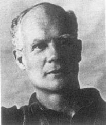
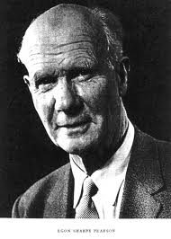
Posts Tagged With: E S Pearson

E.S. Pearson

For a bit more on the statistical philosophy of Egon Sharpe (E.S.) Pearson (11 Aug, 1895-12 June, 1980), I reblog a post from last year. It gets to the question I now call: performance or probativeness?

Are frequentist methods mainly useful to supply procedures which will not err too frequently in some long run? (performance) Or is it the other way round: that the control of long run error properties are of crucial importance for probing causes of the data at hand? (probativeness). I say no to the former and yes to the latter. This I think was also the view of Egon Pearson.

(i) Cases of Type A and Type B

“How far then, can one go in giving precision to a philosophy of statistical inference?” (Pearson 1947, 172)

Pearson considers the rationale that might be given to N-P tests in two types of cases, A and B:

“(A) At one extreme we have the case where repeated decisions must be made on results obtained from some routine procedure…

(B) At the other is the situation where statistical tools are applied to an isolated investigation of considerable importance…?” (ibid., 170)

In cases of type A, long-run results are clearly of interest, while in cases of type B, repetition is impossible and may be irrelevant:

“In other and, no doubt, more numerous cases there is no repetition of the same type of trial or experiment, but all the same we can and many of us do use the same test rules to guide our decision, following the analysis of an isolated set of numerical data. Why do we do this? What are the springs of decision? Is it because the formulation of the case in terms of hypothetical repetition helps to that clarity of view needed for sound judgment?

Or is it because we are content that the application of a rule, now in this investigation, now in that, should result in a long-run frequency of errors in judgment which we control at a low figure?” (Ibid., 173)

Although Pearson leaves this tantalizing question unanswered, claiming, “On this I should not care to dogmatize”, in studying how Pearson treats cases of type B, it is evident that in his view, “the formulation of the case in terms of hypothetical repetition helps to that clarity of view needed for sound judgment” in learning about the particular case at hand.

“Whereas when tackling problem A it is easy to convince the practical man of the value of a probability construct related to frequency of occurrence, in problem B the argument that ‘if we were to repeatedly do so and so, such and such result would follow in the long run’ is at once met by the commonsense answer that we never should carry out a precisely similar trial again.

Nevertheless, it is clear that the scientist with a knowledge of statistical method behind him can make his contribution to a round-table discussion…” (Ibid., 171).

Pearson gives the following example of a case of type B (from his wartime work), where he claims no repetition is intended:

“Example of type B. Two types of heavy armour-piercing naval shell of the same caliber are under consideration; they may be of different design or made by different firms…. Twelve shells of one kind and eight of the other have been fired; two of the former and five of the latter failed to perforate the plate….”(Pearson 1947, 171) 

“Starting from the basis that, individual shells will never be identical in armour-piercing qualities, however good the control of production, he has to consider how much of the difference between (i) two failures out of twelve and (ii) five failures out of eight is likely to be due to this inevitable variability. ..”(Ibid.,)

As a noteworthy aside, Pearson shows that treating the observed difference (between the two proportions) in one way yields an observed significance level of 0.052; treating it differently (along Barnard’s lines), he gets 0.025 as the (upper) significance level. But in scientific cases, Pearson insists, the difference in error probabilities makes no real difference to substantive judgments in interpreting the results. Only in an unthinking, automatic, routine use of tests would it matter:

“Were the action taken to be decided automatically by the side of the 5% level on which the observation point fell, it is clear that the method of analysis used would here be of vital importance. But no responsible statistician, faced with an investigation of this character, would follow an automatic probability rule.” (ibid., 192)

The two analyses correspond to the tests effectively asking different questions, and if we recognize this, says Pearson, different meanings may be appropriately attached.

(ii) Three Steps in the Original construction of Tests

After setting up the test (or null) hypothesis, and the alternative hypotheses against which “we wish the test to have maximum discriminating power” (Pearson 1947, 173), Pearson defines three steps in specifying tests:

“Step 1. We must specify the experimental probability set, the set of results which could follow on repeated application of the random process used in the collection of the data…

Step 2. We then divide this set [of possible results] by a system of ordered boundaries…such that as we pass across one boundary and proceed to the next, we come to a class of results which makes us more and more inclined on the Information  available, to reject the hypothesis tested in favour of alternatives which differ from it by increasing amounts” (Pearson 1966a, 173).

“Step 3. We then, if possible[i], associate with each contour level the chance that, if [the null] is true, a result will occur in random sampling lying beyond that level” (ibid.).

Pearson warns that:

“Although the mathematical procedure may put Step 3 before 2, we cannot put this into operation before we have decided, under Step 2, on the guiding principle to be used in choosing the contour system. That is why I have numbered the steps in this order.” (Ibid. 173).

Strict behavioristic formulations jump from step 1 to step 3, after which one may calculate how the test has in effect accomplished step 2.  However, the resulting test, while having adequate error probabilities, may have an inadequate distance measure and may even be irrelevant to the hypothesis of interest. This is one reason critics can construct howlers that appear to be licensed by N-P methods, and which make their way from time to time into this blog.

So step 3 remains crucial, even for cases of type [B]. There are two reasons: pre-data planning—that’s familiar enough—but secondly, for post-data scrutiny. Post data, step 3 enables determining the capability of the test to have detected various discrepancies, departures, and errors, on which a critical scrutiny of the inferences are based. More specifically, the error probabilities are used to determine how well/poorly corroborated, or how severely tested, various claims are, post-data.

If we can readily bring about statistically significantly higher rates of success with the first type of armour-piercing naval shell than with the second (in the above example), we have evidence the first is superior. Or, as Pearson modestly puts it: the results “raise considerable doubts as to whether the performance of the [second] type of shell was as good as that of the [first]….” (Ibid., 192)[ii]

Still, while error rates of procedures may be used to determine how severely claims have/have not passed they do not automatically do so—hence, again, opening the door to potential howlers that neither Egon nor Jerzy for that matter would have countenanced.

(iii) Neyman Was the More Behavioristic of the Two

Pearson was (rightly) considered to have rejected the more behaviorist leanings of Neyman.

Here’s a snippet from an unpublished letter he wrote to Birnbaum (1974) about the idea that the N-P theory admits of two interpretations: behavioral and evidential:

“I think you will pick up here and there in my own papers signs of evidentiality, and you can say now that we or I should have stated clearly the difference between the behavioral and evidential interpretations. Certainly we have suffered since in the way the people have concentrated (to an absurd extent often) on behavioral interpretations”.

In Pearson’s (1955) response to Fisher (blogged last time):

“To dispel the picture of the Russian technological bogey, I might recall how certain early ideas came into my head as I sat on a gate overlooking an experimental blackcurrant plot….!” (Pearson 1955, 204)

“To the best of my ability I was searching for a way of expressing in mathematical terms what appeared to me to be the requirements of the scientist in applying statistical tests to his data. After contact was made with Neyman in 1926, the development of a joint mathematical theory proceeded much more surely; it was not till after the main lines of this theory had taken shape with its necessary formalization in terms of critical regions, the class of admissible hypotheses, the two sources of error, the power function, etc., that the fact that there was a remarkable parallelism of ideas in the field of acceptance sampling became apparent. Abraham Wald’s contributions to decision theory of ten to fifteen years later were perhaps strongly influenced by acceptance sampling problems, but that is another story.“ (ibid., 204-5).

“It may be readily agreed that in the first Neyman and Pearson paper of 1928, more space might have been given to discussing how the scientific worker’s attitude of mind could be related to the formal structure of the mathematical probability theory….Nevertheless it should be clear from the first paragraph of this paper that we were not speaking of the final acceptance or rejection of a scientific hypothesis on the basis of statistical analysis…. Indeed, from the start we shared Professor Fisher’s view that in scientific enquiry, a statistical test is ‘a means of learning”… (Ibid., 206)

“Professor Fisher’s final criticism concerns the use of the term ‘inductive behavior’; this is Professor Neyman’s field rather than mine.” (Ibid., 207)

__________________________

Aside: It is interesting, given these non-behavioristic leanings that Pearson had earlier worked in acceptance sampling and quality control (from which he claimed to have obtained the term “power”).  From the Cox-Mayo “conversation” (2011, 110):

COX: It is relevant that Egon Pearson had a very strong interest in industrial design and quality control.

MAYO: Yes, that’s surprising, given his evidential leanings and his apparent dis-taste for Neyman’s behavioristic stance. I only discovered that around 10 years ago; he wrote a small book.[iii]

COX: He also wrote a very big book, but all copies were burned in one of the first air raids on London.

Some might find it surprising to learn that it is from this early acceptance sampling work that Pearson obtained the notion of “power”, but I don’t have the quote handy where he said this……

References:

Cox, D. and Mayo, D. G. (2011), “Statistical Scientist Meets a Philosopher of Science: A Conversation,” Rationality, Markets and Morals: Studies at the Intersection of Philosophy and Economics, 2: 103-114.

Pearson, E. S. (1935), The Application of Statistical Methods to Industrial Standardization and Quality Control, London: British Standards Institution.

Pearson, E. S. (1947), “The choice of Statistical Tests illustrated on the Interpretation of Data Classed in a 2×2 Table,” Biometrika 34(1/2): 139-167.

Pearson, E. S. (1955), “Statistical Concepts and Their Relationship to Reality” Journal of the Royal Statistical Society, Series B, (Methodological), 17(2): 204-207.

Neyman, J. and Pearson, E. S. (1928), “On the Use and Interpretation of Certain Test Criteria for Purposes of Statistical Inference, Part I.” Biometrika 20(A): 175-240.