Error Statistics

Gelman est effectivement une erreur statistician

eiffel-tower-design-bill-cannonA reader calls my attention to Andrew Gelman’s blog announcing a talk that he’s giving today in French: “Philosophie et practique de la statistique bayésienne. He blogs:

I’ll try to update the slides a bit since a few years ago, to add some thoughts I’ve had recently about problems with noninformative priors, even in simple settings.

The location of the talk will not be convenient for most of you, but anyone who comes to the trouble of showing up will have the opportunity to laugh at my accent.

P.S. For those of you who are interested in the topic but can’t make it to the talk, I recommend these two papers on my non-inductive Bayesian philosophy:

[2013] Philosophy and the practice of Bayesian statistics (with discussion). British Journal of Mathematical and Statistical Psychology, 8–18. (Andrew Gelman and Cosma Shalizi)
[2013] Rejoinder to discussion. (Andrew Gelman and Cosma Shalizi)

[2011] Induction and deduction in Bayesian data analysis. Rationality, Markets and Morals}, special topic issue “Statistical Science and Philosophy of Science: Where Do (Should) They Meet In 2011 and Beyond?” (Andrew Gelman)

These papers, especially Gelman (2011), are discussed on this blog (in “U-Phils”). Comments by Senn, Wasserman, and Hennig may be found here, and here,with a response here (please use search for more).

As I say in my comments on Gelman and Shalizi, I think Gelman’s position is (or intends to be) inductive– in the sense of being ampliative (going beyond the data)– but simply not probabilist, i.e., not a matter of updating priors. (A blog post is here)[i]. Here’s a snippet from my comments: Continue reading

Categories: Error Statistics, Gelman | Tags: | 17 Comments

(Part 3) Peircean Induction and the Error-Correcting Thesis

C. S. Peirce: 10 Sept, 1839-19 April, 1914

C. S. Peirce: 10 Sept, 1839-19 April, 1914

Last third of “Peircean Induction and the Error-Correcting Thesis”

Deborah G. Mayo
Transactions of the Charles S. Peirce Society 41(2) 2005: 299-319

Part 2 is here.

8. Random sampling and the uniformity of nature

We are now at the point to address the final move in warranting Peirce’s SCT. The severity or trustworthiness assessment, on which the error correcting capacity depends, requires an appropriate link (qualitative or quantitative) between the data and the data generating phenomenon, e.g., a reliable calibration of a scale in a qualitative case, or a probabilistic connection between the data and the population in a quantitative case. Establishing such a link, however, is regarded as assuming observed regularities will persist, or making some “uniformity of nature” assumption—the bugbear of attempts to justify induction.

But Peirce contrasts his position with those favored by followers of Mill, and “almost all logicians” of his day, who “commonly teach that the inductive conclusion approximates to the truth because of the uniformity of nature” (2.775). Inductive inference, as Peirce conceives it (i.e., severe testing) does not use the uniformity of nature as a premise. Rather, the justification is sought in the manner of obtaining data. Justifying induction is a matter of showing that there exist methods with good error probabilities. For this it suffices that randomness be met only approximately, that inductive methods check their own assumptions, and that they can often detect and correct departures from randomness.

… It has been objected that the sampling cannot be random in this sense. But this is an idea which flies far away from the plain facts. Thirty throws of a die constitute an approximately random sample of all the throws of that die; and that the randomness should be approximate is all that is required. (1.94)

Peirce backs up his defense with robustness arguments. For example, in an (attempted) Binomial induction, Peirce asks, “what will be the effect upon inductive inference of an imperfection in the strictly random character of the sampling” (2.728). What if, for example, a certain proportion of the population had twice the probability of being selected? He shows that “an imperfection of that kind in the random character of the sampling will only weaken the inductive conclusion, and render the concluded ratio less determinate, but will not necessarily destroy the force of the argument completely” (2.728). This is particularly so if the sample mean is near 0 or 1. In other words, violating experimental assumptions may be shown to weaken the trustworthiness or severity of the proceeding, but this may only mean we learn a little less.

Yet a further safeguard is at hand:

Nor must we lose sight of the constant tendency of the inductive process to correct itself. This is of its essence. This is the marvel of it. …even though doubts may be entertained whether one selection of instances is a random one, yet a different selection, made by a different method, will be likely to vary from the normal in a different way, and if the ratios derived from such different selections are nearly equal, they may be presumed to be near the truth. (2.729)

Here, the marvel is an inductive method’s ability to correct the attempt at random sampling. Still, Peirce cautions, we should not depend so much on the self-correcting virtue that we relax our efforts to get a random and independent sample. But if our effort is not successful, and neither is our method robust, we will probably discover it. “This consideration makes it extremely advantageous in all ampliative reasoning to fortify one method of investigation by another” (ibid.).

“The Supernal Powers Withhold Their Hands And Let Me Alone”

Peirce turns the tables on those skeptical about satisfying random sampling—or, more generally, satisfying the assumptions of a statistical model. He declares himself “willing to concede, in order to concede as much as possible, that when a man draws instances at random, all that he knows is that he tried to follow a certain precept” (2.749). There might be a “mysterious and malign connection between the mind and the universe” that deliberately thwarts such efforts. He considers betting on the game of rouge et noire: “could some devil look at each card before it was turned, and then influence me mentally” to bet or not, the ratio of successful bets might differ greatly from 0.5. But, as Peirce is quick to point out, this would equally vitiate deductive inferences about the expected ratio of successful bets.

Consider our informal example of weighing with calibrated scales. If I check the properties of the scales against known, standard weights, then I can check if my scales are working in a particular case. Were the scales infected by systematic error, I would discover this by finding systematic mismatches with the known weights; I could then subtract it out in measurements. That scales have given properties where I know the object’s weight indicates they have the same properties when the weights are unknown, lest I be forced to assume that my knowledge or ignorance somehow influences the properties of the scale. More generally, Peirce’s insightful argument goes, the experimental procedure thus confirmed where the measured property is known must work as well when it is unknown unless a mysterious and malign demon deliberately thwarts my efforts. Continue reading

Categories: C.S. Peirce, Error Statistics, phil/history of stat | 6 Comments

(Part 2) Peircean Induction and the Error-Correcting Thesis

C. S. Peirce 9/10/1839 – 4/19/1914

C. S. Peirce
9/10/1839 – 4/19/1914

Continuation of “Peircean Induction and the Error-Correcting Thesis”

Deborah G. Mayo
Transactions of the Charles S. Peirce Society: A Quarterly Journal in American Philosophy, Volume 41, Number 2, 2005, pp. 299-319

Part 1 is here.

There are two other points of confusion in critical discussions of the SCT, that we may note here:

I. The SCT and the Requirements of Randomization and Predesignation

The concern with “the trustworthiness of the proceeding” for Peirce like the concern with error probabilities (e.g., significance levels) for error statisticians generally, is directly tied to their view that inductive method should closely link inferences to the methods of data collection as well as to how the hypothesis came to be formulated or chosen for testing.

This account of the rationale of induction is distinguished from others in that it has as its consequences two rules of inductive inference which are very frequently violated (1.95) namely, that the sample be (approximately) random and that the property being tested not be determined by the particular sample x— i.e., predesignation.

The picture of Peircean induction that one finds in critics of the SCT disregards these crucial requirements for induction: Neither enumerative induction nor H-D testing, as ordinarily conceived, requires such rules. Statistical significance testing, however, clearly does.

Suppose, for example that researchers wishing to demonstrate the benefits of HRT search the data for factors on which treated women fare much better than untreated, and finding one such factor they proceed to test the null hypothesis:

H0: there is no improvement in factor F (e.g. memory) among women treated with HRT.

Having selected this factor for testing solely because it is a factor on which treated women show impressive improvement, it is not surprising that this null hypothesis is rejected and the results taken to show a genuine improvement in the population. However, when the null hypothesis is tested on the same data that led it to be chosen for testing, it is well known, a spurious impression of a genuine effect easily results. Suppose, for example, that 20 factors are examined for impressive-looking improvements among HRT-treated women, and the one difference that appears large enough to test turns out to be significant at the 0.05 level. The actual significance level—the actual probability of reporting a statistically significant effect when in fact the null hypothesis is true—is not 5% but approximately 64% (Mayo 1996, Mayo and Kruse 2001, Mayo and Cox 2006). To infer the denial of H0, and infer there is evidence that HRT improves memory, is to make an inference with low severity (approximately 0.36).

II Understanding the “long-run error correcting” metaphor

Discussions of Peircean ‘self-correction’ often confuse two interpretations of the ‘long-run’ error correcting metaphor, even in the case of quantitative induction: (a) Asymptotic self-correction (as n approaches ∞): In this construal, it is imagined that one has a sample, say of size n=10, and it is supposed that the SCT assures us that as the sample size increases toward infinity, one gets better and better estimates of some feature of the population, say the mean. Although this may be true, provided assumptions of a statistical model (e.g., the Binomial) are met, it is not the sense intended in significance-test reasoning nor, I maintain, in Peirce’s SCT. Peirce’s idea, instead, gives needed insight for understanding the relevance of ‘long-run’ error probabilities of significance tests to assess the reliability of an inductive inference from a specific set of data, (b) Error probabilities of a test: In this construal, one has a sample of size n, say 10, and imagines hypothetical replications of the experiment—each with samples of 10. Each sample of 10 gives a single value of the test statistic d(X), but one can consider the distribution of values that would occur in hypothetical repetitions (of the given type of sampling). The probability distribution of d(X) is called the sampling distribution, and the correct calculation of the significance level is an example of how tests appeal to this distribution: Thanks to the relationship between the observed d(x) and the sampling distribution of d(X), the former can be used to reliably probe the correctness of statistical hypotheses (about the procedure) that generated the particular 10-fold sample. That is what the SCT is asserting.

It may help to consider a very informal example. Suppose that weight gain is measured by 10 well-calibrated and stable methods, possibly using several measuring instruments and the results show negligible change over a test period of interest. This may be regarded as grounds for inferring that the individual’s weight gain is negligible within limits set by the sensitivity of the scales. Why? While it is true that by averaging more and more weight measurements, i.e., an eleventh, twelfth, etc., one would get asymptotically close to the true weight, that is not the rationale for the particular inference. The rationale is rather that the error probabilistic properties of the weighing procedure (the probability of ten-fold weighings erroneously failing to show weight change) inform one of the correct weight in the case at hand, e.g., that a 0 observed weight increase passes the “no-weight gain” hypothesis with high severity. Continue reading

Categories: Bayesian/frequentist, C.S. Peirce, Error Statistics, Statistics | 5 Comments

Peircean Induction and the Error-Correcting Thesis (Part I)

C. S. Peirce: 10 Sept, 1839-19 April, 1914

C. S. Peirce: 10 Sept, 1839-19 April, 1914

Today is C.S. Peirce’s birthday. I hadn’t blogged him before, but he’s one of my all time heroes. You should read him: he’s a treasure chest on essentially any topic. I’ll blog the main sections of a (2005) paper over the next few days. It’s written for a very general philosophical audience; the statistical parts are pretty informal. Happy birthday Peirce.

Peircean Induction and the Error-Correcting Thesis
Deborah G. Mayo
Transactions of the Charles S. Peirce Society: A Quarterly Journal in American Philosophy, Volume 41, Number 2, 2005, pp. 299-319

Peirce’s philosophy of inductive inference in science is based on the idea that what permits us to make progress in science, what allows our knowledge to grow, is the fact that science uses methods that are self-correcting or error-correcting:

Induction is the experimental testing of a theory. The justification of it is that, although the conclusion at any stage of the investigation may be more or less erroneous, yet the further application of the same method must correct the error. (5.145)

Inductive methods—understood as methods of experimental testing—are justified to the extent that they are error-correcting methods. We may call this Peirce’s error-correcting or self-correcting thesis (SCT):

Self-Correcting Thesis SCT: methods for inductive inference in science are error correcting; the justification for inductive methods of experimental testing in science is that they are self-correcting.

Peirce’s SCT has been a source of fascination and frustration. By and large, critics and followers alike have denied that Peirce can sustain his SCT as a way to justify scientific induction: “No part of Peirce’s philosophy of science has been more severely criticized, even by his most sympathetic commentators, than this attempted validation of inductive methodology on the basis of its purported self-correctiveness” (Rescher 1978, p. 20).

In this paper I shall revisit the Peircean SCT: properly interpreted, I will argue, Peirce’s SCT not only serves its intended purpose, it also provides the basis for justifying (frequentist) statistical methods in science. While on the one hand, contemporary statistical methods increase the mathematical rigor and generality of Peirce’s SCT, on the other, Peirce provides something current statistical methodology lacks: an account of inductive inference and a philosophy of experiment that links the justification for statistical tests to a more general rationale for scientific induction. Combining the mathematical contributions of modern statistics with the inductive philosophy of Peirce, sets the stage for developing an adequate justification for contemporary inductive statistical methodology.

2. Probabilities are assigned to procedures not hypotheses

Peirce’s philosophy of experimental testing shares a number of key features with the contemporary (Neyman and Pearson) Statistical Theory: statistical methods provide, not means for assigning degrees of probability, evidential support, or confirmation to hypotheses, but procedures for testing (and estimation), whose rationale is their predesignated high frequencies of leading to correct results in some hypothetical long-run. A Neyman and Pearson (NP) statistical test, for example, instructs us “To decide whether a hypothesis, H, of a given type be rejected or not, calculate a specified character, x0, of the observed facts; if x> x0 reject H; if x< x0 accept H.” Although the outputs of N-P tests do not assign hypotheses degrees of probability, “it may often be proved that if we behave according to such a rule … we shall reject H when it is true not more, say, than once in a hundred times, and in addition we may have evidence that we shall reject H sufficiently often when it is false” (Neyman and Pearson, 1933, p.142).[i]

The relative frequencies of erroneous rejections and erroneous acceptances in an actual or hypothetical long run sequence of applications of tests are error probabilities; we may call the statistical tools based on error probabilities, error statistical tools. In describing his theory of inference, Peirce could be describing that of the error-statistician:

The theory here proposed does not assign any probability to the inductive or hypothetic conclusion, in the sense of undertaking to say how frequently that conclusion would be found true. It does not propose to look through all the possible universes, and say in what proportion of them a certain uniformity occurs; such a proceeding, were it possible, would be quite idle. The theory here presented only says how frequently, in this universe, the special form of induction or hypothesis would lead us right. The probability given by this theory is in every way different—in meaning, numerical value, and form—from that of those who would apply to ampliative inference the doctrine of inverse chances. (2.748)

The doctrine of “inverse chances” alludes to assigning (posterior) probabilities in hypotheses by applying the definition of conditional probability (Bayes’s theorem)—a computation requires starting out with a (prior or “antecedent”) probability assignment to an exhaustive set of hypotheses:

If these antecedent probabilities were solid statistical facts, like those upon which the insurance business rests, the ordinary precepts and practice [of inverse probability] would be sound. But they are not and cannot be statistical facts. What is the antecedent probability that matter should be composed of atoms? Can we take statistics of a multitude of different universes? (2.777)

For Peircean induction, as in the N-P testing model, the conclusion or inference concerns a hypothesis that either is or is not true in this one universe; thus, assigning a frequentist probability to a particular conclusion, other than the trivial ones of 1 or 0, for Peirce, makes sense only “if universes were as plentiful as blackberries” (2.684). Thus the Bayesian inverse probability calculation seems forced to rely on subjective probabilities for computing inverse inferences, but “subjective probabilities” Peirce charges “express nothing but the conformity of a new suggestion to our prepossessions, and these are the source of most of the errors into which man falls, and of all the worse of them” (2.777).

Hearing Pierce contrast his view of induction with the more popular Bayesian account of his day (the Conceptualists), one could be listening to an error statistician arguing against the contemporary Bayesian (subjective or other)—with one important difference. Today’s error statistician seems to grant too readily that the only justification for N-P test rules is their ability to ensure we will rarely take erroneous actions with respect to hypotheses in the long run of applications. This so called inductive behavior rationale seems to supply no adequate answer to the question of what is learned in any particular application about the process underlying the data. Peirce, by contrast, was very clear that what is really wanted in inductive inference in science is the ability to control error probabilities of test procedures, i.e., “the trustworthiness of the proceeding”. Moreover it is only by a faulty analogy with deductive inference, Peirce explains, that many suppose that inductive (synthetic) inference should supply a probability to the conclusion: “… in the case of analytic inference we know the probability of our conclusion (if the premises are true), but in the case of synthetic inferences we only know the degree of trustworthiness of our proceeding (“The Probability of Induction” 2.693).

Knowing the “trustworthiness of our inductive proceeding”, I will argue, enables determining the test’s probative capacity, how reliably it detects errors, and the severity of the test a hypothesis withstands. Deliberately making use of known flaws and fallacies in reasoning with limited and uncertain data, tests may be constructed that are highly trustworthy probes in detecting and discriminating errors in particular cases. This, in turn, enables inferring which inferences about the process giving rise to the data are and are not warranted: an inductive inference to hypothesis H is warranted to the extent that with high probability the test would have detected a specific flaw or departure from what H asserts, and yet it did not.

3. So why is justifying Peirce’s SCT thought to be so problematic?

You can read Section 3 here. (it’s not necessary for understanding the rest).

4. Peircean induction as severe testing

… [I]nduction, for Peirce, is a matter of subjecting hypotheses to “the test of experiment” (7.182).

The process of testing it will consist, not in examining the facts, in order to see how well they accord with the hypothesis, but on the contrary in examining such of the probable consequences of the hypothesis … which would be very unlikely or surprising in case the hypothesis were not true. (7.231)

When, however, we find that prediction after prediction, notwithstanding a preference for putting the most unlikely ones to the test, is verified by experiment,…we begin to accord to the hypothesis a standing among scientific results.

This sort of inference it is, from experiments testing predictions based on a hypothesis, that is alone properly entitled to be called induction. (7.206)

While these and other passages are redolent of Popper, Peirce differs from Popper in crucial ways. Peirce, unlike Popper, is primarily interested not in falsifying claims but in the positive pieces of information provided by tests, with “the corrections called for by the experiment” and with the hypotheses, modified or not, that manage to pass severe tests. For Popper, even if a hypothesis is highly corroborated (by his lights), he regards this as at most a report of the hypothesis’ past performance and denies it affords positive evidence for its correctness or reliability. Further, Popper denies that he could vouch for the reliability of the method he recommends as “most rational”—conjecture and refutation. Indeed, Popper’s requirements for a highly corroborated hypothesis are not sufficient for ensuring severity in Peirce’s sense (Mayo 1996, 2003, 2005). Where Popper recoils from even speaking of warranted inductions, Peirce conceives of a proper inductive inference as what had passed a severe test—one which would, with high probability, have detected an error if present.

In Peirce’s inductive philosophy, we have evidence for inductively inferring a claim or hypothesis H when not only does H “accord with” the data x; but also, so good an accordance would very probably not have resulted, were H not true. In other words, we may inductively infer H when it has withstood a test of experiment that it would not have withstood, or withstood so well, were H not true (or were a specific flaw present). This can be encapsulated in the following severity requirement for an experimental test procedure, ET, and data set x.

Hypothesis H passes a severe test with x iff (firstly) x accords with H and (secondly) the experimental test procedure ET would, with very high probability, have signaled the presence of an error were there a discordancy between what H asserts and what is correct (i.e., were H false).

The test would “have signaled an error” by having produced results less accordant with H than what the test yielded. Thus, we may inductively infer H when (and only when) H has withstood a test with high error detecting capacity, the higher this probative capacity, the more severely H has passed. What is assessed (quantitatively or qualitatively) is not the amount of support for H but the probative capacity of the test of experiment ET (with regard to those errors that an inference to H is declaring to be absent)……….

You can read the rest of Section 4 here.

5. The path from qualitative to quantitative induction

In my understanding of Peircean induction, the difference between qualitative and quantitative induction is really a matter of degree, according to whether their trustworthiness or severity is quantitatively or only qualitatively ascertainable. This reading not only neatly organizes Peirce’s typologies of the various types of induction, it underwrites the manner in which, within a given classification, Peirce further subdivides inductions by their “strength”.

(I) First-Order, Rudimentary or Crude Induction

Consider Peirce’s First Order of induction: the lowest, most rudimentary form that he dubs, the “pooh-pooh argument”. It is essentially an argument from ignorance: Lacking evidence for the falsity of some hypothesis or claim H, provisionally adopt H. In this very weakest sort of induction, crude induction, the most that can be said is that a hypothesis would eventually be falsified if false. (It may correct itself—but with a bang!) It “is as weak an inference as any that I would not positively condemn” (8.237). While uneliminable in ordinary life, Peirce denies that rudimentary induction is to be included as scientific induction. Without some reason to think evidence of H‘s falsity would probably have been detected, were H false, finding no evidence against H is poor inductive evidence for H. H has passed only a highly unreliable error probe. Continue reading

Categories: Bayesian/frequentist, C.S. Peirce, Error Statistics, Statistics | 6 Comments

First blog: “Did you hear the one about the frequentist…”? and “Frequentists in Exile”

metablog old fashion typewriterDear Reader: Tonight marks the 2-year anniversary of this blog; so I’m reblogging my very first posts from 9/3/11 here and here (from the rickety old blog site)*. (One was the “about”.) The current blog was included once again in the top 50 statistics blogs. Amazingly, I have received e-mails from different parts of the world describing experimental recipes for the special concoction we exiles favor!  (Mine is here.) If you can fly over to the Elbar Room, please join us: I’m treating everyone to doubles of Elbar Grease!  Thanks for reading and contributing! D. G. Mayo

(*The old blogspot is a big mix; it was before Rejected blogs. Yes, I still use this old typewriter [ii])

“Overheard at the Comedy Club at the Bayesian Retreat” 9/3/11 by D. Mayoimages-3

“Did you hear the one about the frequentist . . .

  • “who claimed that observing “heads” on a biased coin that lands heads with probability .05 is evidence of a statistically significant improvement over the standard treatment of diabetes, on the grounds that such an event occurs with low probability (.05)?”

or

  • “who defended the reliability of his radiation reading, despite using a broken radiometer, on the grounds that most of the time he uses one that works, so on average he’s pretty reliable?”

Such jests may work for an after-dinner laugh, but if it turns out that, despite being retreads of “straw-men” fallacies, they form the basis of why some reject frequentist methods, then they are not such a laughing matter.   But surely the drubbing of frequentist methods could not be based on a collection of howlers, could it?  I invite the curious reader to stay and find out.

If we are to take the criticisms seriously, and put to one side the possibility that they are deliberate distortions of frequentist statistical methods, we need to identify their sources. To this end I consider two interrelated areas around which to organize foundational issues in statistics: (1) the roles of probability in induction and inference, and (2) the nature and goals of statistical inference in science or learning. Frequentist sampling statistics, which I prefer to call “error statistics,” continues to be raked over the coals in the foundational literature, but with little scrutiny of the presuppositions about goals and methods, without which the criticisms lose all force.

First, there is the supposition that an adequate account must assign degrees of probability to hypotheses, an assumption often called probabilism. Second, there is the assumption that the main, if not the only, goal of error-statistical methods is to evaluate long-run error rates.   Given the wide latitude with which some critics define “controlling long-run error,” it is not surprising to find them arguing that (i) error statisticians approve of silly methods, and/or (ii) rival (e.g., Bayesian) accounts also satisfy error statistical demands. Absent this sleight of hand, Bayesian celebrants would have to go straight to the finale of their entertainment hour: a rousing rendition of “There’s No Theorem Like Bayes’s Theorem.”

Never mind that frequentists have responded to these criticisms, they keep popping up (verbatim) in many Bayesian textbooks and articles on philosophical foundations. The difficulty of articulating a statistical philosophy that fully explains the basis for both (i)  insisting on error-statistical guarantees, while (ii) avoiding pathological examples in practice, has turned many a frequentist away from venturing into foundational battlegrounds.  Some even concede the distorted perspectives drawn from overly literal and radical expositions of what Fisher, Neyman, and Pearson “really thought”.  Many others just find the “statistical wars” distasteful.

Here is where I view my contribution—as a philosopher of science—to the long-standing debate: not merely to call attention to the howlers that pass as legitimate criticisms of frequentist error statistics, but also to sketch the main lines of an alternative statistical philosophy within which to better articulate the roles and value of frequentist tools. Let me be clear that I do not consider this the only philosophical framework for frequentist statistics—different terminology could do as well.  I will consider myself successful if I can provide one way of building, or one standpoint from which to build, a frequentist, error- statistical philosophy.

But given this is a blog, I shall be direct and to the point: I hope to cultivate the interests of others who might want to promote intellectual honesty within a generally very lopsided philosophical debate.  I will begin with the first entry to the comedy routine, as it is put forth by leading Bayesians……

___________________________________________

“Frequentists in Exile” 9/3/11 by D. Mayo

Confronted with the position that “arguments for this personalistic theory were so persuasive that anything to any extent inconsistent with that theory should be discarded” (Cox 2006, 196), frequentists might have seen themselves in a kind of exile when it came to foundations, even those who had been active in the dialogues of an earlier period [i].  Sometime around the late 1990s there were signs that this was changing.  Regardless of the explanation, the fact that it did occur and is occurring is of central importance to statistical philosophy.

Now that Bayesians have stepped off their a priori pedestal, it may be hoped that a genuinely deep scrutiny of the frequentist and Bayesian accounts will occur.  In some corners of practice it appears that frequentist error statistical foundations are being discovered anew.  Perhaps frequentist foundations, never made fully explicit, but at most lying deep below the ocean floor, are finally being disinterred.  But let’s learn from some of the mistakes in the earlier attempts to understand it.  With this goal I invite you to join me in some deep water drilling, here as I cast about on my Isle of Elba.

Cox, D. R. (2006), Principles of Statistical Inference, CUP.

________________________________________________

[i] Yes, that’s the Elba connection: Napolean’s exile (from which he returned to fight more battles).

[ii] I have discovered a very reliable antique typewriter shop in Oxford that was able to replace the two missing typewriter keys. So long as my “ribbons” and carbon sheets don’t run out, I’m set.

Categories: Comedy, Error Statistics | Tags: , , , | 40 Comments

Gelman’s response to my comment on Jaynes

3-d red yellow puzzle people (E&I)Gelman responds to the comment[i] I made on my 8/31/13 post:
Popper and Jaynes
Posted by Andrew on 3 September 2013
Deborah Mayo quotes me as saying, “Popper has argued (convincingly, in my opinion) that scientific inference is not inductive but deductive.” She then follows up with:

Gelman employs significance test-type reasoning to reject a model when the data sufficiently disagree.

Now, strictly speaking, a model falsification, even to inferring something as weak as “the model breaks down,” is not purely deductive, but Gelman is right to see it as about as close as one can get, in statistics, to a deductive falsification of a model. But where does that leave him as a Jaynesian?

My reply:

I was influenced by reading a toy example from Jaynes’s book where he sets up a model (for the probability of a die landing on each of its six sides) based on first principles, then presents some data that contradict the model, then expands the model.

I’d seen very little of this sort of this reasoning before in statistics! In physics it’s the standard way to go: you set up a model based on physical principles and some simplifications (for example, in a finite-element model you assume the various coefficients aren’t changing over time, and you assume stability within each element), then if the model doesn’t quite work, you figure out what went wrong and you make it more realistic.

But in statistics we weren’t usually seeing this. Instead, model checking typically was placed in the category of “hypothesis testing,” where the rejection was the goal. Models to be tested were straw man, build up only to be rejected. You can see this, for example, in social science papers that list research hypotheses that are not the same as the statistical “hypotheses” being tested. A typical research hypothesis is “Y causes Z,” with the corresponding statistical hypothesis being “Y has no association with Z after controlling for X.” Jaynes’s approach—or, at least, what I took away from Jaynes’s presentation—was more simpatico to my way of doing science. And I put a lot of effort into formalizing this idea, so that the kind of modeling I talk and write about can be the kind of modeling I actually do.

I don’t want to overstate this—as I wrote earlier, Jaynes is no guru—but I do think this combination of model building and checking is important. Indeed, just as a chicken is said to be an egg’s way of making another egg, we can view inference as a way of sharpening the implications of an assumed model so that it can better be checked.

P.S. In response to Larry’s post here, let me give a quick +1 to this comment and also refer to this post, which remains relevant 3 years later.

I still don’t see how one learns about falsification from Jaynes when he alleges that the entailment of x from H disappears once H is rejected. But put that aside. In my quote from Gelman 2011, he was alluding to simple significance tests–without an alternative–for checking consistency of a model; whereas, he’s now saying what he wants is to infer an alternative model, and furthermore suggests one doesn’t see this in statistical hypotheses tests. But of course Neyman-Pearson testing always has an alternative, and even Fisherian simple significance tests generally indicate a direction of departure. However, neither type of statistical test method would automatically license going directly from a rejection of one statistical hypotheses to inferring an alternative model that was constructed to account for the misfit. A parametric discrepancy,δ, from a null may be indicated if the test very probably would not have resulted in so large an observed difference, were such a discrepancy absent (i.e., when the inferred alternative passes severely). But I’m not sure Gelman is limiting himself to such alternatives.

As I wrote in a follow-up comment: “there’s no warrant to infer a particular model that happens to do a better job fitting the data x–at least on x alone. Insofar as there are many alternatives that could patch things up, an inference to one particular alternative fails to pass with severity. I don’t understand how it can be that some of the critics of the (bad) habit of some significance testers to move from rejecting the null to a particular alternative, nevertheless seem prepared to allow this in Bayesian model testing. But maybe they carry out further checks down the road; I don’t claim to really get the methods of correcting Bayesian priors (as part of a model)”

A published discussion of Gelman and Shalizi on this matter is here.

[i] My comment was:

” If followers of Jaynes agree with [one of the commentators] (and Jaynes, apparently) that as soon as H is falsified, the grounds on which the test was based disappear!—a position that is based on a fallacy– then I’m confused as to how Andrew Gelman can claim to follow Jaynes at all. 
“Popper has argued (convincingly, in my opinion) that scientific inference is not inductive but deductive…” (Gelman, 2011, bottom p. 71).
Gelman employs significance test-type reasoning to reject a model when the data sufficiently disagree.
 Now, strictly speaking, a model falsification, even to inferring something as weak as “the model breaks down,” is not purely deductive, but Gelman is right to see it as about as close as one can get, in statistics, to a deductive falsification of a model. But where does that leave him as a Jaynesian? Perhaps he’s not one of the ones in Paul’s Jaynes/Bayesian audience who is laughing, but is rather shaking his head?”
Categories: Error Statistics, significance tests, Statistics | 9 Comments

Is Bayesian Inference a Religion?

Reblogging a stimulating post from the Normal Deviate!

normaldeviate's avatarNormal Deviate

Time for a provocative post.

There is a nice YouTube video with Tony O’Hagan interviewing Dennis Lindley. Of course, Dennis is a legend and his impact on the field of statistics is huge.

At one point, Tony points out that some people liken Bayesian inference to a religion. Dennis claims this is false. Bayesian inference, he correctly points out, starts with some basic axioms and then the rest follows by deduction. This is logic, not religion.

I agree that the mathematics of Bayesian inference is based on sound logic. But, with all due respect, I think Dennis misunderstood the question. When people say that “Bayesian inference is like a religion,” they are not referring to the logic of Bayesian inference. They are referring to how adherents of Bayesian inference behave.

(As an aside, detractors of Bayesian inference do not deny the correctness of the logic. They just don’t think…

View original post 371 more words

Categories: Error Statistics | 23 Comments

Overheard at the comedy hour at the Bayesian retreat-2 years on

mic-comedy-clubIt’s nearly two years since I began this blog, and some are wondering if I’ve covered all the howlers thrust our way? Sadly, no. So since it’s Saturday night here at the Elba Room, let’s listen in on one of the more puzzling fallacies–one that I let my introductory logic students spot…

“Did you hear the one about significance testers sawing off their own limbs?

‘Suppose we decide that the effect exists; that is, we reject [null hypothesis] H0. Surely, we must also reject probabilities conditional on H0, but then what was the logical justification for the decision? Orthodox logic saws off its own limb.’ “

Ha! Ha! By this reasoning, no hypothetical testing or falsification could ever occur. As soon as H is falsified, the grounds for falsifying disappear! If H: all swans are white, then if I see a black swan, H is falsified. But according to this critic, we can no longer assume the deduced prediction from H! What? The entailment from a hypothesis or model H to x, whether it is statistical or deductive, does not go away after the hypothesis or model H is rejected on grounds that the prediction is not born out.[i] When particle physicists deduce that the events could not be due to background alone, the statistical derivation (to what would be expected under H: background alone) does not get sawed off when H is denied!images-2

The above quote is from Jaynes (p. 524) writing on the pathologies of “orthodox” tests. How does someone writing a great big book on “the logic of science” get this wrong? To be generous, we may assume that in the heat of criticism, his logic takes a wild holiday. Unfortunately, I’ve heard several of his acolytes repeat this. There’s a serious misunderstanding of how hypothetical reasoning works: 6 lashes, and a pledge not to uncritically accept what critics say, however much you revere them.
______

Jaynes, E. T. 2003. Probability Theory: The Logic of Science. Cambridge: Cambridge University Press.

[i]Of course there is also no warrant for inferring an alternative hypothesis, unless it is a non-null warranted with severity—even if the alternative entails the existence of a real effect. (Statistical significance is not substantive significance—it is by now cliché . Search this blog for fallacies of rejection.)

A few previous comedy hour posts:

(09/03/11) Overheard at the comedy hour at the Bayesian retreat
(4/4/12) Jackie Mason: Fallacy of Rejection and the Fallacy of Nouvelle Cuisine
(04/28/12) Comedy Hour at the Bayesian Retreat: P-values versus Posteriors

(05/05/12) Comedy Hour at the Bayesian (Epistemology) Retreat: Highly Probable vs Highly Probed
(09/03/12) After dinner Bayesian comedy hour…. (1 year anniversary)
(09/08/12) Return to the comedy hour…(on significance tests)
(04/06/13) Who is allowed to cheat? I.J. Good and that after dinner comedy hour….
(04/27/13) Getting Credit (or blame) for Something You Didn’t Do (BP oil spill, comedy hour)

Categories: Comedy, Error Statistics, Statistics | 22 Comments

A critical look at “critical thinking”: deduction and induction

images-1I’m cleaning away some cobwebs around my old course notes, as I return to teaching after 2 years off (since I began this blog). The change of technology alone over a mere 2 years (at least here at Super Tech U) might be enough to earn me techno-dinosaur status: I knew “Blackboard” but now it’s “Scholar” of which I know zilch. The course I’m teaching is supposed to be my way of bringing “big data” into introductory critical thinking in philosophy! No one can be free of the “sexed up term for statistics,” Nate Silver told us (here and here), and apparently all the college Deans & Provosts have followed suit. Of course I’m (mostly) joking; and it was my choice.

Anyway, the course is a nostalgic trip back to critical thinking. Stepping back from the grown-up metalogic and advanced logic I usually teach, hop-skipping over baby logic, whizzing past toddler and infant logic…. and arriving at something akin to what R.A. Fisher dubbed “the study of the embryology of knowledge” (1935, 39) (a kind of ‘fetal logic’?) which, in its very primitiveness, actually demands a highly sophisticated analysis. In short, it’s turning out to be the same course I taught nearly a decade ago! (but with a new book and new twists). But my real point is that the hodge-podge known as “critical thinking,” were it seriously considered, requires getting to grips with some very basic problems that we philosophers, with all our supposed conceptual capabilities, have left unsolved. (I am alluding to Gandenberger‘s remark). I don’t even think philosophers are working on the problem (these days). (Are they?)

I refer, of course, to our inadequate understanding of how to relate deductive and inductive inference, assuming the latter to exist (which I do)—whether or not one chooses to call its study a “logic”[i]. [That is, even if one agrees with the Popperians that the only logic is deductive logic, there may still be such a thing as a critical scrutiny of the approximate truth of premises, without which no inference is ever detached even from a deductive argument. This is also required for Popperian corroboration or well-testedness.]

We (and our textbooks) muddle along with vague attempts to see inductive arguments as more or less parallel to deductive ones, only with probabilities someplace or other. I’m not saying I have easy answers, I’m saying I need to invent a couple of new definitions in the next few days that can at least survive the course. Maybe readers can help.

______________________

I view ‘critical thinking’ as developing methods for critically evaluating the (approximate) truth or adequacy of the premises which may figure in deductive arguments. These methods would themselves include both deductive and inductive or “ampliative” arguments. Deductive validity is a matter of form alone, and so philosophers are stuck on the idea that inductive logic would have a formal rendering as well. But this simply is not the case. Typical attempts are arguments with premises that take overly simple forms:

If all (or most) J’s were observed to be K’s, then the next J will be a K, at least with a probability p.

To evaluate such a claim (essentially the rule of enumerative induction) requires context-dependent information (about the nature and selection of the K and J properties, their variability, the “next” trial, and so on). Besides, most interesting ampliative inferences are to generalizations and causal claims, not mere predictions to the next J. The problem isn’t that an algorithm couldn’t evaluate such claims, but that the evaluation requires context-dependent information as to how the ampliative leap can go wrong. Yet our most basic texts speak as if potentially warranted inductive arguments are like potentially sound deductive arguments, more or less. But it’s not easy to get the “more or less” right, for any given example, while still managing to say anything systematic and general. That is essentially the problem…..
______________________

The age-old definition of argument that we all learned from Irving Copi still serves: a group of statements, one of which (the conclusion) is claimed to follow from one or more others (the premises) which are regarded as supplying evidence for the truth of that one. This is written:

P1, P2,…Pn/ ∴ C.

In a deductively valid argument, if the premises are all true then, necessarily, the conclusion is true. To use the “⊨” (double turnstile) symbol:

 P1, P2,…Pn ⊨  C.

Does this mean:

 P1, P2,…Pn/ ∴ necessarily C?

No, because we do not detach “necessarily C”, which would suggest C was a necessary claim (i.e., true in all possible worlds). “Necessarily” qualifies “⊨”, the very relationship between premises and conclusion:

It’s logically impossible to have all true premises and a false conclusion, on pain of logical contradiction.

We should see it (i.e., deductive validity) as qualifying the process of “inferring,” as opposed to the “inference” that is detached–the statement  placed to the right of “⊨”. A valid argument is a procedure of inferring that is 100% reliable, in the sense that if the premises are all true, then 100% of the time the conclusion is true.

Deductively Valid Argument: Three equivalent expressions:

(D-i) If the premises are all true, then necessarily, the conclusion is true.
(I.e., if the conclusion is false, then (necessarily) one of premises is false.)

(D-ii) It’s (logically) impossible for the premises to be true and the conclusion false.
(I.e., to have the conclusion false with the premises true leads to a logical contradiction, A & ~A.)

(D-iii) The argument maps true premises into a true conclusion with 100% reliability.
(I.e., if the premises are all true, then 100% of the time the conclusion is true).

(Deductively) Sound argument:  deductively valid + premises are true/approximately true.

All of this is baby logic; but with so-called inductive arguments, terms are not so clear-cut. (“Embryonic logic” demands, at times, more sophistication than grown-up logic.) But maybe the above points can help…

________

With an inductive argument, the conclusion goes beyond the premises. So it’s logically possible for all the premises to be true and the conclusion false.

Notice that if one had characterized deductive validity as

(a)  P1, P2,…Pn ⊨ necessarily C,

then it would be an easy slide to seeing inductively inferring as:

(b)  P1, P2,…Pnprobably C.

But (b) is wrongheaded, I say, for the same reason (a) is. Nevertheless, (b) (or something similar) is found in many texts. We (philosophers) should stop foisting ampliative inference into the deductive mould. So, here I go trying out some decent parallels:

In all of the following, “true” will mean “true or approximately true”.

An inductive argument (to inference C) is strong or potentially severe only if any of the following (equivalent claims) hold [iii]

(I-i) If the conclusion is false, then very probably at least one of the premises is false.

(I-ii) It’s improbable that the premises are all true while the conclusion false.

(I-iii) The argument leads from true premises to a true conclusion with high reliability (i.e., if the premises are all true then (1-a)% of the time, the conclusion is true).

To get the probabilities to work, the premises and conclusion must refer to “generic” claims of the type, but this is the case for deductive arguments as well (else their truth values wouldn’t be altering). However, the basis for the [I-i through I-iii] requirement, in any of its forms, will not be formal; it will demand a contingent or empirical ground. Even after these are grounded, the approximate truth of the premises will be required. Otherwise, it’s only potentially severe. (This is parallel to viewing a valid deductive argument as potentially sound.)

We get the following additional parallel:

Deductively unsound argument:

Denial of D-(i), (D-ii), or (D-iii): it’s logically possible for all its premises to be true and the conclusion false.
OR
One or more of its premises are false.

Inductively weak inference: insevere grounds for C

Denial of I-(i), (ii), or (iii): Premises would be fairly probable even if C is false.
OR
Its premises are false (not true to a sufficient approximation)

There’s still some “winking” going on, and I’m sure I’ll have to tweak this. What do you think?

Fully aware of how the fuzziness surrounding inductive inference has non-trivially (adversely) influenced the entire research program in philosophy of induction, I’ll want to rethink some elements from scratch, this time around….

______________

So I’m back in my Thebian palace high atop the mountains in Blacksburg, Virginia. The move from looking out at the Empire state building to staring at endless mountain ranges is… calming.[iv]

References:

[i] I do, following Peirce, but it’s an informal not a formal logic (using the terms strictly).

[ii]The double turnstile denotes the “semantic consequence” relationship; the single turnstyle, the syntatic (deducibility) relationship. But some students are not so familiar with “turnstiles”.

[iii]I intend these to function equivalently.

[iv] Someone asked me “what’s the biggest difference I find in coming to the rural mountains from living in NYC?” I think the biggest contrast is the amount of space. Not just that I live in a large palace, there’s the tremendous width of grocery aisles: 3 carts wide rather than 1.5 carts wide. I hate banging up against carts in NYC, but this feels like a major highway!

Copi, I.  (1956). Introduction to Logic. New York: Macmillan.

Fisher, R.A.  (1935). The Design of Experiments.  Edinburgh: Oliver & Boyd.


Categories: critical thinking, Severity, Statistics | 28 Comments

Blog contents: July, 2013

metablog old fashion typewriter(7/3) Phil/Stat/Law: 50 Shades of gray between error and fraud
(7/6) Bad news bears: ‘Bayesian bear’ rejoinder–reblog mashup
(7/10) PhilStatLaw: Reference Manual on Scientific Evidence (3d ed) on Statistical Significance (Schachtman)
(7/11) Is Particle Physics Bad Science? (memory lane)
(7/13) Professor of Philosophy Resigns over Sexual Misconduct (rejected post)
(7/14) Stephen Senn: Indefinite irrelevance
(7/17) Phil/Stat/Law: What Bayesian prior should a jury have? (Schachtman)
(7/19) Msc Kvetch: A question on the Martin-Zimmerman case we do not hear
(7/20) Guest Post: Larry Laudan. Why Presuming Innocence is Not a Bayesian Prior
(7/23) Background Knowledge: Not to Quantify, But To Avoid Being Misled By,Subjective Beliefs
(7/26) New Version: On the Birnbaum argument for the SLP: Slides for JSM talk

Categories: Error Statistics | Leave a comment

A. Spanos: Egon Pearson’s Neglected Contributions to Statistics

may-4-8-aris-spanos-e2809contology-methodology-in-statistical-modelinge2809dWith permission from my colleague Aris Spanos, I reblog his (8/18/12): “Egon Pearson’s Neglected Contributions to Statistics“. It illuminates a different area of E.S.P’s work than my posts here and here.

    Egon Pearson (11 August 1895 – 12 June 1980), is widely known today for his contribution in recasting of Fisher’s significance testing into the Neyman-Pearson (1933) theory of hypothesis testing. Occasionally, he is also credited with contributions in promoting statistical methods in industry and in the history of modern statistics; see Bartlett (1981). What is rarely mentioned is Egon’s early pioneering work on:

(i) specification: the need to state explicitly the inductive premises of one’s inferences,

(ii) robustness: evaluating the ‘sensitivity’ of inferential procedures to departures from the Normality assumption, as well as

(iii) Mis-Specification (M-S) testing: probing for potential departures from the Normality  assumption.

Arguably, modern frequentist inference began with the development of various finite sample inference procedures, initially by William Gosset (1908) [of the Student’s t fame] and then Fisher (1915, 1921, 1922a-b). These inference procedures revolved around a particular statistical model, known today as the simple Normal model:

Xk ∽ NIID(μ,σ²), k=1,2,…,n,…             (1)

where ‘NIID(μ,σ²)’ stands for ‘Normal, Independent and Identically Distributed with mean μ and variance σ²’. These procedures include the ‘optimal’ estimators of μ and σ², Xbar and s², and the pivotal quantities:

(a) τ(X) =[√n(Xbar- μ)/s] ∽ St(n-1),  (2)

(b) v(X) =[(n-1)s²/σ²] ∽ χ²(n-1),        (3)

where St(n-1) and χ²(n-1) denote the Student’s t and chi-square distributions with (n-1) degrees of freedom.

The question of ‘how these inferential results might be affected when the Normality assumption is false’ was originally raised by Gosset in a letter to Fisher in 1923:

“What I should like you to do is to find a solution for some other population than a normal one.”  (Lehmann, 1999)

He went on to say that he tried the rectangular (uniform) distribution but made no progress, and he was seeking Fisher’s help in tackling this ‘robustness/sensitivity’ problem. In his reply that was unfortunately lost, Fisher must have derived the sampling distribution of τ(X), assuming some skewed distribution (possibly log-Normal). We know this from Gosset’s reply:

“I like the result for z [τ(X)] in the case of that horrible curve you are so fond of. I take it that in skew curves the distribution of z is skew in the opposite direction.”  (Lehmann, 1999)

After this exchange Fisher was not particularly receptive to Gosset’s requests to address the problem of working out the implications of non-Normality for the Normal-based inference procedures; t, chi-square and F tests.

In contrast, Egon Pearson shared Gosset’s concerns about the robustness of Normal-based inference results (a)-(b) to non-Normality, and made an attempt to address the problem in a series of papers in the late 1920s and early 1930s. This line of research for Pearson began with a review of Fisher’s 2nd edition of the 1925 book, published in Nature, and dated June 8th, 1929.  Pearson, after praising the book for its path breaking contributions, dared raise a mild criticism relating to (i)-(ii) above:

“There is one criticism, however, which must be made from the statistical point of view. A large number of tests are developed upon the assumption that the population sampled is of ‘normal’ form. That this is the case may be gathered from a very careful reading of the text, but the point is not sufficiently emphasised. It does not appear reasonable to lay stress on the ‘exactness’ of tests, when no means whatever are given of appreciating how rapidly they become inexact as the population samples diverge from normality.” (Pearson, 1929a)

Fisher reacted badly to this criticism and was preparing an acerbic reply to the ‘young pretender’ when Gosset jumped into the fray with his own letter in Nature, dated July 20th, in an obvious attempt to moderate the ensuing fight. Gosset succeeded in tempering Fisher’s reply, dated August 17th, forcing him to provide a less acerbic reply, but instead of addressing the ‘robustness/sensitivity’ issue, he focused primarily on Gosset’s call to address ‘the problem of what sort of modification of my tables for the analysis of variance would be required to adapt that process to non-normal distributions’. He described that as a hopeless task. This is an example of Fisher’s genious when cornered by an insightful argument. He sidestepped the issue of ‘robustness’ to departures from Normality, by broadening it – alluding to other possible departures from the ID assumption – and rendering it a hopeless task, by focusing on the call to ‘modify’ the statistical tables for all possible non-Normal distributions; there is an infinity of potential modifications!

Egon Pearson recognized the importance of stating explicitly the inductive premises upon which the inference results are based, and pressed ahead with exploring the robustness issue using several non-Normal distributions within the Pearson family. His probing was based primarily on simulation, relying on tables of pseudo-random numbers; see Pearson and Adyanthaya (1928, 1929), Pearson (1929b, 1931). His broad conclusions were that the t-test:

τ0(X)=|[√n(X-bar- μ0)/s]|, C1:={x: τ0(x) > cα},    (4)

for testing the hypotheses:

H0: μ = μ0 vs. H1: μ ≠ μ0,                                             (5)

is relatively robust to certain departures from Normality, especially when the underlying distribution is symmetric, but the ANOVA test is rather sensitive to such departures! He continued this line of research into his 80s; see Pearson and Please (1975).

Perhaps more importantly, Pearson (1930) proposed a test for the Normality assumption based on the skewness and kurtosis coefficients: a Mis-Specification (M-S) test. Ironically, Fisher (1929) provided the sampling distributions of the sample skewness and kurtosis statistics upon which Pearson’s test was based. Pearson continued sharpening his original M-S test for Normality, and his efforts culminated with the D’Agostino and Pearson (1973) test that is widely used today; see also Pearson et al. (1977). The crucial importance of testing Normality stems from the fact that it renders the ‘robustness/sensitivity’ problem manageable. The test results can be used to narrow down the possible departures one needs to worry about. They can also be used to suggest ways to respecify the original model.

After Pearson’s early publications on the ‘robustness/sensitivity’ problem Gosset realized that simulation alone was not effective enough to address the question of robustness, and called upon Fisher, who initially rejected Gosset’s call by saying ‘it was none of his business’, to derive analytically the implications of non-Normality using different distributions:

“How much does it [non-Normality] matter? And in fact that is your business: none of the rest of us have the slightest chance of solving the problem: we can play about with samples [i.e. perform simulation studies], I am not belittling E. S. Pearson’s work, but it is up to you to get us a proper solution.” (Lehmann, 1999).

In this passage one can discern the high esteem with which Gosset held Fisher for his technical ability. Fisher’s reply was rather blunt:

“I do not think what you are doing with nonnormal distributions is at all my business, and I doubt if it is the right approach. … Where I differ from you, I suppose, is in regarding normality as only a part of the difficulty of getting data; viewed in this collection of difficulties I think you will see that it is one of the least important.”

It’s clear from this that Fisher understood the problem of how to handle departures from Normality more broadly than his contemporaries. His answer alludes to two issues that were not well understood at the time:

(a) departures from the other two probabilistic assumptions (IID) have much more serious consequences for Normal-based inference than Normality, and

(b) deriving the consequences of particular forms of non-Normality on the reliability of Normal-based inference, and proclaiming a procedure enjoys a certain level of ‘generic’ robustness, does not provide a complete answer to the problem of dealing with departures from the inductive premises.

In relation to (a) it is important to note that the role of ‘randomness’, as it relates to the IID assumptions, was not well understood until the 1940s, when the notion of non-IID was framed in terms of explicit forms of heterogeneity and dependence pertaining to stochastic processes. Hence, the problem of assessing departures from IID was largely ignored at the time, focusing almost exclusively on departures from Normality. Indeed, the early literature on nonparametric inference retained the IID assumptions and focused on inference procedures that replace the Normality assumption with indirect distributional assumptions pertaining to the ‘true’ but unknown f(x), like the existence of certain moments, its symmetry, smoothness, continuity and/or differentiability, unimodality, etc. ; see Lehmann (1975). It is interesting to note that Egon Pearson did not consider the question of testing the IID assumptions until his 1963 paper.

In relation to (b), when one poses the question ‘how robust to non-Normality is the reliability of inference based on a t-test?’ one ignores the fact that the t-test might no longer be the ‘optimal’ test under a non-Normal distribution. This is because the sampling distribution of the test statistic and the associated type I and II error probabilities depend crucially on the validity of the statistical model assumptions. When any of these assumptions are invalid, the relevant error probabilities are no longer the ones derived under the original model assumptions, and the optimality of the original test is called into question. For instance, assuming that the ‘true’ distribution is uniform (Gosset’s rectangular):

Xk ∽ U(a-μ,a+μ),   k=1,2,…,n,…        (6)

where f(x;a,μ)=(1/(2μ)), (a-μ) ≤ x ≤ (a+μ), μ > 0,

how does one assess the robustness of the t-test? One might invoke its generic robustness to symmetric non-Normal distributions and proceed as if the t-test is ‘fine’ for testing the hypotheses (5). A more well-grounded answer will be to assess the discrepancy between the nominal (assumed) error probabilities of the t-test based on (1) and the actual ones based on (6). If the latter approximate the former ‘closely enough’, one can justify the generic robustness. These answers, however, raise the broader question of what are the relevant error probabilities? After all, the optimal test for the hypotheses (5) in the context of (6), is no longer the t-test, but the test defined by:

w(X)=|{(n-1)([X[1] +X[n]]-μ0)}/{[X[1]-X[n]]}|∽F(2,2(n-1)),   (7)

with a rejection region C1:={x: w(x) > cα},  where (X[1], X[n]) denote the smallest and the largest element in the ordered sample (X[1], X[2],…, X[n]), and F(2,2(n-1)) the F distribution with 2 and 2(n-1) degrees of freedom; see Neyman and Pearson (1928). One can argue that the relevant comparison error probabilities are no longer the ones associated with the t-test ‘corrected’ to account for the assumed departure, but those associated with the test in (7). For instance, let the t-test have nominal and actual significance level, .05 and .045, and power at μ10+1, of .4 and .37, respectively. The conventional wisdom will call the t-test robust, but is it reliable (effective) when compared with the test in (7) whose significance level and power (at μ1) are say, .03 and .9, respectively?

A strong case can be made that a more complete approach to the statistical misspecification problem is:

(i) to probe thoroughly for any departures from all the model assumptions using trenchant M-S tests, and if any departures are detected,

(ii) proceed to respecify the statistical model by choosing a more appropriate model with a view to account for the statistical information that the original model did not.

Admittedly, this is a more demanding way to deal with departures from the underlying assumptions, but it addresses the concerns of Gosset, Egon Pearson, Neyman and Fisher much more effectively than the invocation of vague robustness claims; see Spanos (2010).

References

Bartlett, M. S. (1981) “Egon Sharpe Pearson, 11 August 1895-12 June 1980,” Biographical Memoirs of Fellows of the Royal Society, 27: 425-443.

D’Agostino, R. and E. S. Pearson (1973) “Tests for Departure from Normality. Empirical Results for the Distributions of b₂ and √(b₁),” Biometrika, 60: 613-622.

Fisher, R. A. (1915) “Frequency distribution of the values of the correlation coefficient in samples from an indefinitely large population,” Biometrika, 10: 507-521.

Fisher, R. A. (1921) “On the “probable error” of a coefficient of correlation deduced from a small sample,” Metron, 1: 3-32.

Fisher, R. A. (1922a) “On the mathematical foundations of theoretical statistics,” Philosophical Transactions of the Royal Society A, 222, 309-368.

Fisher, R. A. (1922b) “The goodness of fit of regression formulae, and the distribution of regression coefficients,” Journal of the Royal Statistical Society, 85: 597-612.

Fisher, R. A. (1925) Statistical Methods for Research Workers, Oliver and Boyd, Edinburgh.

Fisher, R. A. (1929), “Moments and Product Moments of Sampling Distributions,” Proceedings of the London Mathematical Society, Series 2, 30: 199-238.

Neyman, J. and E. S. Pearson (1928) “On the use and interpretation of certain test criteria for purposes of statistical inference: Part I,” Biometrika, 20A: 175-240.

Neyman, J. and E. S. Pearson (1933) “On the problem of the most efficient tests of statistical hypotheses”, Philosophical Transanctions of the Royal Society, A, 231: 289-337.

Lehmann, E. L. (1975) Nonparametrics: statistical methods based on ranks, Holden-Day, San Francisco.

Lehmann, E. L. (1999) “‘Student’ and Small-Sample Theory,” Statistical Science, 14: 418-426.

Pearson, E. S. (1929a) “Review of ‘Statistical Methods for Research Workers,’ 1928, by Dr. R. A. Fisher”, Nature, June 8th, pp. 866-7.

Pearson, E. S. (1929b) “Some notes on sampling tests with two variables,” Biometrika, 21: 337-60.

Pearson, E. S. (1930) “A further development of tests for normality,” Biometrika, 22: 239-49.

Pearson, E. S. (1931) “The analysis of variance in cases of non-normal variation,” Biometrika, 23: 114-33.

Pearson, E. S. (1963) “Comparison of tests for randomness of points on a line,” Biometrika, 50: 315-25.

Pearson, E. S. and N. K. Adyanthaya (1928) “The distribution of frequency constants in small samples from symmetrical populations,” Biometrika, 20: 356-60.

Pearson, E. S. and N. K. Adyanthaya (1929) “The distribution of frequency constants in small samples from non-normal symmetrical and skew populations,” Biometrika, 21: 259-86.

Pearson, E. S. and N. W. Please (1975) “Relations between the shape of the population distribution and the robustness of four simple test statistics,” Biometrika, 62: 223-241.

Pearson, E. S., R. B. D’Agostino and K. O. Bowman (1977) “Tests for departure from normality: comparisons of powers,” Biometrika, 64: 231-246.

Spanos, A. (2010) “Akaike-type Criteria and the Reliability of Inference: Model Selection vs. Statistical Model Specification,” Journal of Econometrics, 158: 204-220.

Student (1908), “The Probable Error of the Mean,” Biometrika, 6: 1-25.

Categories: phil/history of stat, Statistics, Testing Assumptions | Tags: , , , | 5 Comments

What did Nate Silver just say? Blogging the JSM

imagesNate Silver gave his ASA Presidential talk to a packed audience (with questions tweeted[i]). Here are some quick thoughts—based on scribbled notes (from last night). Silver gave a list of 10 points that went something like this (turns out there were 11):

1. statistics are not just numbers

2. context is needed to interpret data

3. correlation is not causation

4. averages are the most useful tool

5. human intuitions about numbers tend to be flawed and biased

6. people misunderstand probability

7. we should be explicit about our biases and (in this sense) should be Bayesian?

8. complexity is not the same as not understanding

9. being in the in crowd gets in the way of objectivity

10. making predictions improves accountability

Just to comment on #7, I don’t know if this is a brand new philosophy of Bayesianism, but his position went like this: Journalists and others are incredibly biased, they view data through their prior conceptions, wishes, goals, and interests, and you cannot expect them to be self-critical enough to be aware of, let alone be willing to expose, their propensity toward spin, prejudice, etc. Silver said the reason he favors the Bayesian philosophy (yes he used the words “philosophy” and “epistemology”) is that people should be explicit about disclosing their biases. I have three queries: (1) If we concur that people are so inclined to see the world through their tunnel vision, what evidence is there that they are able/willing to be explicit about their biases? (2) If priors are to be understood as the way to be explicit about one’s biases, shouldn’t they be kept separate from the data rather than combined with them? (3) I don’t think this is how Bayesians view Bayesianism or priors—is it? Subjective Bayesians, I thought, view priors as representing prior or background information about the statistical question of interest; but Silver sees them as admissions of prejudice, bias or what have you. As a confession of bias, I’d be all for it—though I think people may be better at exposing other’s biases than their own. Only thing: I’d need an entirely distinct account of warranted inference from data.

This does possibly explain some inexplicable remarks in Silver’s book to the effect that R.A. Fisher denied, excluded, or overlooked human biases since he disapproved of adding subjective prior beliefs to data in scientific contexts. Is Silver just about to recognize/appreciate the genius of Fisher (and others) in developing techniques consciously designed to find things out despite knowledge gaps, variability, and human biases? Or not?

Share your comments and/or links to other blogs discussing his talk (which will surely be posted if it isn’t already). Fill in gaps if you were there—I was far away… (See also my previous post blogging the JSM). Photo on 8-4-13 at 3.40 PM


[i] What was the point of this, aside from permitting questions to be cherry picked? (It would have been fun to see ALL the queries tweeted.) The ones I heard were limited to: how can we make statistics more attractive, who is your favorite journalist, favorite baseball player, and so on. But I may have missed some, I left before the end.

For a follow-up post including an 11th bullet that I’d missed, see here. My first post on JSM13 (8/5/13) was here.

Categories: Error Statistics, Statistics | 42 Comments

At the JSM: 2013 International Year of Statistics

Photo on 8-4-13 at 3.40 PM“2013 is the International Year of Statistics” the JSM (Joint Statistical Meetings) brochures ring out! What does it mean?  Whatever it is, it’s exciting! Errorstatistics.com never took up this question, but it’s been on some of the blogs in my “Blog bagel”. So, Since I’m at the JSM here in Montreal, I may report on any clues. Please share your comments. I’m not a statistician, but a philosopher of science, and of inductive-statistical inference much more generally. So I have no dog in this fight, as they say. (Or do I? ) On the other hand, I have often rued “the decline of late in the lively and long-standing exchange between philosophers of science and statisticians” (see this post). [i] (We did have that one parody on “big data or pig data”.)

I know from Larry Wasserman (normaldeviate) that the “year of” label grows, at least in part, to help prevent Statistical Science being eclipsed by the fashionable “Big Data” crowd. In one blog he even spoke of “the end of statistics”. “Aren’t We Data Science?” Marie Davidian, president of the ASA, asks in a recent AmStatNews article.[ii] Davidian worries, correctly I’ve no doubt, that Big Dadaists may be collecting data with “little appreciation for the power of design principle. Statisticians could propel major advances through developments of ‘experimental design for the 21st century’!”.  This recalls Stan Young’s recent post:

Until relatively recently, the microarray samples were not sent through assay equipment in random order. Clinical trial statisticians at GSK insisted that the samples go through assay in random order. Rather amazingly the data became less messy and p-values became more orderly. The story is given here:
 http://blog.goldenhelix.com/?p=322. 
Essentially all the microarray data pre-2010 is unreliable…..So often the problem is not with p-value technology, but with the design and conduct of the study.

So without statistical design principles, they may have wasted a decade!

Back to the JSM, I see they’ve even invited pollster Nate Silver to give the AMA presidential address. I thought he was more baseball stat expert/pundit/pollster than statistician, but some are calling him an “analytics rock star”. Never mind that there’s at least one extremely strange chapter (8) in his popular book (The Signal and the Noise). Here’s an excerpt from Wasserman’s review, which he titles:  “Nate Silver is a Frequentist: Review of The signal and the noise”:


I have one complaint. Silver is a big fan of Bayesian inference, which is fine. Unfortunately, he falls into that category I referred to a few posts ago. He confuses ‘Bayesian inference’ with ‘using Bayes’ theorem.’ His description of frequentist inference is terrible. He seems to equate frequentist inference with Fisherian significance testing, most using Normal distributions. Either he learned statistics from a bad book or he hangs out with statisticians with a significant anti-frequentist bias. Have no doubt about it: Nate Silver is a frequentist.[iii] (Wasserman)

I didn’t discuss Silver’s book on this blog, but looking up a few comments I made on other blogs, (e.g.,on a Gelman blog reviewing Silver), I see I am a bit less generous than Wasserman: “Frequentists, Silver alleges, go around reporting hypotheses like toads predict earthquakes and other “manifestly ridiculous” findings that are licensed by significance testing and data dredged correlations. (Silver, 253). But it is the frequentist who prevents such spurious correlations…. “  (Mayo) So Silver’s criticisms of frequents are way off base.  I was also slightly aghast at his Fisher ridicule and I poke fun at his “All-You-Need is Bayesian cheerleading. The simple use of Bayes Theorem solves all problems (he seems not to realize they too require statistical models)” I wrote.  It’s hard to tell if he’s just reporting or chiming in with those who advocate that schools stop teaching frequentist methods. Some statistical self-inflicted wounds perhaps? The other chapters look interesting, though I didn’t get too much further…(The Bayesian examples are all ordinary frequentist updating, it appears.)   If I can, I’ll go to Silver’s talk.

[i] In that post I wrote: “Philosophy of statistical science not only deals with the philosophical foundations of statistics but also questions about the nature of and justification for inductive-statistical learning more generally. So it is ironic that just as philosophy of science is striving to immerse itself in and be relevant to scientific practice, that statistical science and philosophy of science—so ahead of their time in combining the work of philosophers and practicing scientists—should see such dialogues become rather rare.  (See special topic here.)” (Mayo)

[ii] Some of the turf battles I hear about appear to reflect less substance than style (i.e., people being galvanized to use the latest meme in funding opportunities). Even in philosophy, the dept. head asked us to try and work it in.   In my view, rather than suggesting “Plato and Big Data”, they should be asking to highlight interconnections between statistical evidence, critical thinking, logic, ethics,  philosophy of science, and epistemology. That would advance our courses.

[iii] For example, Wasserman says, in his review of Silver:

One of the most important tests of a forecast — I would argue that it is the single most important one — is called calibration. Out of all the times you said there was a 40 percent chance of rain, how often did rain actually occur? If over the long run, it really did rain about 40 percent of the time, that means your forecasts were well calibrated.  (Wasserman)

Categories: Error Statistics | 5 Comments

New Version: On the Birnbaum argument for the SLP: Slides for my JSM talk

Picture 216 1mayo In my latest formulation of the controversial Birnbaum argument for the strong likelihood principle (SLP), I introduce a new symbol \Rightarrow  
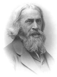
to represent a function from a given experiment-outcome pair, (E,z) to a generic inference implication.  This should clarify my argument (see my new paper).

(E,z) \Rightarrow InfrE(z) is to be read “the inference implication from outcome z in experiment E” (according to whatever inference type/school is being discussed).

A draft of my slides for the Joint Statistical Meetings JSM in Montreal next week are right after the abstract. Comments are very welcome.

Interested readers may search this blog for quite a lot of discussion of the SLP (e.g., here and here) including links to the central papers, “U-Phils” by others (e.g., here, here, and here), and amusing notes (e.g., Don’t Birnbaumize that experiment my friend, and Midnight with Birnbaum).

On the Birnbaum Argument for the Strong Likelihood Principle

Abstract

An essential component of inference based on familiar frequentist notions p-values, significance and confidence levels, is the relevant sampling distribution (hence the term sampling theory). This feature results in violations of a principle known as the strong likelihood principle (SLP), the focus of this paper. In particular, if outcomes x* and y* from experiments E1 and E2 (both with unknown parameter θ), have different probability models f1, f2, then even though f1(x*; θ) = cf2(y*; θ) for all θ, outcomes x* and y* may have different implications for an inference about θ. Although such violations stem from considering outcomes other than the one observed, we argue, this does not require us to consider experiments other than the one performed to produce the data. David Cox (1958) proposes the Weak Conditionality Principle (WCP) to justify restricting the space of relevant repetitions. The WCP says that once it is known which Ei produced the measurement, the assessment should be in terms of the properties of the particular Ei.      

The surprising upshot of Allan Birnbaum’s (1962) argument is that the SLP appears to follow from applying the WCP in the case of mixtures, and so uncontroversial a principle as sufficiency (SP). But this would preclude the use of sampling distributions. The goal of this article is to provide a new clarification and critique of Birnbaum’s argument. Although his argument purports that [(WCP and SP) entails SLP], we show how data may violate the SLP while holding both the WCP and SP. Such cases directly refute [WCP entails SLP].

Comments, questions, errors are welcome.

Full paper can be found here: http://arxiv-web3.library.cornell.edu/abs/1302.7021

Categories: Error Statistics, Statistics, strong likelihood principle | 20 Comments

Background Knowledge: Not to Quantify, But To Avoid Being Misled By, Subjective Beliefs

drapery6A low-powered statistical analysis of this blog—nearing its 2-year anniversary!—reveals that the topic to crop up most often—either front and center, or lurking in the bushes–is that of “background information”. The following was one of my early posts, back in Oct.30, 2011:

October 30, 2011 (London). Increasingly, I am discovering that one of the biggest sources of confusion about the foundations of statistics has to do with what it means or should mean to use “background knowledge” and “judgment” in making statistical and scientific inferences. David Cox and I address this in our “Conversation” in RMM (2011); it is one of the three or four topics in that special volume that I am keen to take up.

Insofar as humans conduct science and draw inferences, and insofar as learning about the world is not reducible to a priori deductions, it is obvious that “human judgments” are involved. True enough, but too trivial an observation to help us distinguish among the very different ways judgments should enter according to contrasting inferential accounts. When Bayesians claim that frequentists do not use or are barred from using background information, what they really mean is that frequentists do not use prior probabilities of hypotheses, at least when those hypotheses are regarded as correct or incorrect, if only approximately. So, for example, we would not assign relative frequencies to the truth of hypotheses such as (1) prion transmission is via protein folding without nucleic acid, or (2) the deflection of light is approximately 1.75” (as if, as Pierce puts it, “universes were as plenty as blackberries”). How odd it would be to try to model these hypotheses as themselves having distributions: to us, statistical hypotheses assign probabilities to outcomes or values of a random variable.

However, quite a lot of background information goes into designing, carrying out, and analyzing inquiries into hypotheses regarded as correct or incorrect. For a frequentist, that is where background knowledge enters. There is no reason to suppose that the background required in order sensibly to generate, interpret, and draw inferences about H should—or even can—enter through prior probabilities for H itself! Of course, presumably, Bayesians also require background information in order to determine that “data x” have been observed, to determine how to model and conduct the inquiry, and to check the adequacy of statistical models for the purposes of the inquiry. So the Bayesian prior only purports to add some other kind of judgment, about the degree of belief in H. It does not get away from the other background judgments that frequentists employ.

This relates to a second point that came up in our conversation when Cox asked, “Do we want to put in a lot of information external to the data, or as little as possible?” Continue reading

Categories: Background knowledge, Error Statistics | Tags: , | Leave a comment

Why I am not a “dualist” in the sense of Sander Greenland

Janus--2face

This post picks up, and continues, an exchange that began with comments on my June 14 blogpost (between Sander Greenland, Nicole Jinn, and I). My new response is at the end. The concern is how to expose and ideally avoid some of the well known flaws and foibles in statistical inference, thanks to gaps between data and statistical inference, and between statistical inference and substantive claims. I am not rejecting the use of multiple methods in the least (they are highly valuable when one method is capable of detecting or reducing flaws in one or more others). Nor am I speaking of classical dualism in metaphysics (which I also do not espouse). I begin with Greenland’s introduction of this idea in his comment… (For various earlier comments, see the post.)

Sander Greenland 

. I sense some confusion of criticism of the value of tests as popular tools vs. criticism of their logical foundation. I am a critic in the first, practical category, who regards the adoption of testing outside of narrow experimental programs as an unmitigated disaster, resulting in publication bias, prosecutor-type fallacies, and affirming the consequent fallacies throughout the health and social science literature. Even though testing can in theory be used soundly, it just hasn’t done well in practice in these fields. This could be ascribed to human failings rather than failings of received testing theories, but I would require any theory of applied statistics to deal with human limitations, just as safety engineering must do for physical products. I regard statistics as having been woefully negligent of cognitive psychology in this regard. In particular, widespread adoption and vigorous defense of a statistical method or philosophy is no more evidence of its scientific value than widespread adoption and vigorous defense of a religion is evidence of its scientific value. 
That should bring us to alternatives. I am aware of no compelling data showing that other approaches would have done better, but I do find compelling the arguments that at least some of the problems would have been mitigated by teaching a dualist approach to statistics, in which every procedure must be supplied with both an accurate frequentist and an accurate Bayesian interpretation, if only to reduce prevalent idiocies like interpreting a two-sided P-value as “the” posterior probability of a point null hypothesis.

 Nicole Jinn
 (to Sander Greenland)

 What exactly is this ‘dualist’ approach to teaching statistics and why does it mitigate the problems, as you claim? (I am increasingly interested in finding more effective ways to teach/instruct others in various age groups about statistics.)
I have a difficult time seeing how effective this ‘dualist’ way of teaching could be for the following reason: the Bayesian and frequentist approaches are vastly different in their aims and the way they see statistics being used in (natural or social) science, especially when one looks more carefully at the foundations of each methodology (e.g., disagreements about where exactly probability enters into inference, or about what counts as relevant information). Hence, it does not make sense (to me) to supply both types of interpretation to the same data and the same research question! Instead, it makes more sense (from a teaching perspective) to demonstrate a Bayesian interpretation for one experiment, and a frequentist interpretation for another experiment, in the hopes of getting at the (major) differences between the two methodologies.

Mayo

Sander. Thanks for your comment. 
Interestingly, I think the conglomeration of error statistical tools are the ones most apt at dealing with human limitations and foibles: they give piecemeal methods to ask one question at a time (e.g., would we be mistaken to suppose there is evidence of any effect at all? mistaken about how large? about iid assumptions? about possible causes? about implications for distinguishing any theories?). The standard Bayesian apparatus requires setting out a complete set of hypotheses that might arise, plus prior probabilities in each of them (or in “catchall” hypotheses), as well as priors in the model…and after this herculean task is complete, there is a purely deductive update: being deductive it never goes beyond the givens. Perhaps the data will require a change in your prior—this is what you must have believed before, since otherwise you find your posterior unacceptable—thereby encouraging the very self-sealing inferences we all claim to deplore. Continue reading

Categories: Bayesian/frequentist, Error Statistics, P-values, Statistics | 21 Comments

Anything Tests Can do, CIs do Better; CIs Do Anything Better than Tests?* (reforming the reformers cont.)

Having reblogged the 5/17/12 post on “reforming the reformers” yesterday, I thought I should reblog its follow-up: 6/2/12.

Consider again our one-sided Normal test T+, with null H0: μ < μ0 vs μ >μ0  and  μ0 = 0,  α=.025, and σ = 1, but let n = 25. So M is statistically significant only if it exceeds .392. Suppose M (the sample mean) just misses significance, say

Mo = .39.

The flip side of a fallacy of rejection (discussed before) is a fallacy of acceptance, or the fallacy of misinterpreting statistically insignificant results.  To avoid the age-old fallacy of taking a statistically insignificant result as evidence of zero (0) discrepancy from the null hypothesis μ =μ0, we wish to identify discrepancies that can and cannot be ruled out.  For our test T+, we reason from insignificant results to inferential claims of the form:

μ < μ0 + γ

Fisher continually emphasized that failure to reject was not evidence for the null.  Neyman, we saw, in chastising Carnap, argued for the following kind of power analysis:

Neymanian Power Analysis (Detectable Discrepancy Size DDS): If data x are not statistically significantly different from H0, and the power to detect discrepancy γ is high (low), then x constitutes good (poor) evidence that the actual effect is < γ. (See 11/9/11 post).

By taking into account the actual x0, a more nuanced post-data reasoning may be obtained.

“In the Neyman-Pearson theory, sensitivity is assessed by means of the power—the probability of reaching a preset level of significance under the assumption that various alternative hypotheses are true. In the approach described here, sensitivity is assessed by means of the distribution of the random variable P, considered under the assumption of various alternatives. “ (Cox and Mayo 2010, p. 291):

This may be captured in :

FEV(ii): A moderate p-value is evidence of the absence of a discrepancy d from Ho only if there is a high probability the test would have given a worse fit with H0 (i.e., a smaller p value) were a discrepancy d to exist. (Mayo and Cox 2005, 2010, 256).

This is equivalently captured in the Rule of Acceptance (Mayo (EGEK) 1996, and in the severity interpretation for acceptance, SIA, Mayo and Spanos (2006, p. 337):

SIA: (a): If there is a very high probability that [the observed difference] would have been larger than it is, were μ > μ1, then μ < μ1 passes the test with high severity,…

But even taking tests and CIs just as we find them, we see that CIs do not avoid the fallacy of acceptance: they do not block erroneous construals of negative results adequately. Continue reading

Categories: CIs and tests, Error Statistics, reformers, Statistics | Tags: , , , , , , , | Leave a comment

K. Staley: review of Error & Inference

kent-staleyK. W. Staley
Associate Professor
Department of Philosophy,
Saint Louis University

(Almost) All about error


BOOK REVIEW Metascience (2012) 21:709–713 DOI 10.1007/s11016-011-9618-1E & I Cover 2
Deborah G. Mayo and Aris Spanos (eds): Error and inference: Recent exchanges on experimental reasoning, reliability, objectivity, and rationality. New York: Cambridge University Press, 2010, xvii+419 pp

The ERROR’06 (experimental reasoning, reliability, objectivity, and rationality) conference held at Virginia Tech aimed to advance the discussion of some central themes in philosophy of science debated by Deborah Mayo and her more-or-less friendly critics over the years. The volume here reviewed brings together the contributions of these critics and Mayo’s responses to them (with Mayo’s collaborator Aris Spanos). (I helped with the organization of the conference and, with Mayo and Jean Miller, edited a separate collection of workshop papers that were presented there, published as a special issue of Synthese.) My review will focus on a couple of themes I hope to be of interest to a broad philosophical audience, then turn more briefly to an overview of the entire collection. The discussions in Error and Inference (E&I) are indispensable for understanding several current issues regarding the methodology of science.

The remarkably useful introductory chapter lays out the broad themes of the volume and discusses ‘‘The Error-Statistical Philosophy’’. Here, Mayo and Spanos provide the most succinct and non-technical account of the error-statistical approach that has yet been published, a feature that alone should commend this text to anyone who has found it difficult to locate a reading on error statistics suitable for use in teaching.

Mayo holds that the central question for a theory of evidence is not the degree to which some observation E confirms some hypothesis H but how well-probed for error a hypothesis H is by a testing procedure T that results in data x0. This reorientation has far-reaching consequences for Mayo’s approach to philosophy of science. On this approach, addressing the question of when data ‘‘provide good evidence for or a good test of’’ a hypothesis requires attention to characteristics of the process by means of which the data are used to bear on the hypothesis. Mayo identifies the starting point from which her account is developed as the ‘‘Weak Severity Principle’’ (WSP):

Data x0 do not provide good evidence for hypothesis H if x0 results from a test procedure with a very low probability or capacity of having uncovered the falsity of H (even if H is incorrect). (21)

The weak severity principle is then developed into the full severity principle (SP), according to which ‘‘data x0 provide a good indication of or evidence for hypothesis H (just) to the extent that test T has severely passed H with x0’’ where H passes a severe test T with x0 if x0 ‘‘agrees with’’ H and ‘‘with very high probability, test T would have produced a result that accords less well with H than doesx0, if H were false or incorrect’’ (22). This principle constitutes the heart of the error-statistical account of evidence, and E&I, by including some of the most important critiques of the principle, provides a forum in which Mayo and Spanos attempt to correct misunderstandings of the principle and to clarify its meaning and application.

The appearance in the WSP of the disjunctive phrase ‘‘a very low probability or capacity’’ (my emphasis) indicates a point central to much of this clarificatory work. The error-statistical account is resolutely frequentist in its construal of probability. It is commonly held (including by some frequentists) that the rationale for frequentist statistical methods lies exclusively in the fact that they can sometimes be shown to have low error rates in the long run. Throughout E&I, Mayo insists that this ‘‘behaviorist rationale’’ is not applicable when it comes to evaluating a particular body of data in order to determine what inferences may be warranted. That evaluation rests upon thinking about the particular data and the inference at hand in light of the capacity of the test to reveal potential errors in the inference drawn. Frequentist probabilities are part of how one models the error-detecting capacities of the process. As Mayo explains in a later chapter co-authored with David Cox, tests of hypotheses function analogously to measuring instruments: ‘‘Just as with the use of measuring instruments, applied to a specific case, we employ the performance features to make inferences about aspects of the particular thing that is measured, aspects that the measuring tool is appropriately capable of revealing’’ (257).

One of the most fascinating exchanges in E&I concerns the role of severe testing in the appraisal of ‘‘large-scale’’ theories. According to Mayo, theory appraisal proceeds by a ‘‘piecemeal’’ process of severe probing for specific ways in which a theory might be in error. She illustrates this with the history of experimental tests of theories of gravity, emphasizing Clifford Will’s parametrized post-Newtonian (PPN) framework, by means of which all metric theories of gravity can be represented in their weak-field, slow-motion limits by means of ten parameters. Experimental work on gravity theories then severely tests hypotheses about the values of those parameters. Rather than attempting to confirm or probabilify the general theory of relativity (GTR), the aim is to learn about the ways in which GTR might be in error, more generally to ‘‘measure how far off what a given theory says about a phenomenon can be from what a ‘correct’ theory would need to say about it’’ (55).

Alan Chalmers and Alan Musgrave both challenge this view. According to Chalmers, no general theory, whether ‘‘low level’’ or ‘‘high level’’, can pass a severe test because the content of theories surpasses whatever empirical evidence supports them. As a consequence, Chalmers argues, Mayo’s severe-testing account of scientific inference must be incomplete because even low-level experimental testing sometimes demands relying on general theoretical claims. Similarly, Musgrave accuses Mayo of holding that (general) theories are not tested by ‘‘testing their consequences’’, but that ‘‘all that we really test are the consequences’’ (105), leaving her with ‘‘nothing to say’’ about the assessment, adoption, or rejection of general theories (106). Continue reading

Categories: Error Statistics, Statistics | Tags: , | 1 Comment

Does statistics have an ontology? Does it need one? (draft 2)

questionmark pinkChance, rational beliefs, decision, uncertainty, probability, error probabilities, truth, random sampling, resampling, opinion, expectations. These are some of the concepts we bandy about by giving various interpretations to mathematical statistics, to statistical theory, and to probabilistic models. But are they real? The question of “ontology” asks about such things, and given the “Ontology and Methodology” conference here at Virginia Tech (May 4, 5), I’d like to get your thoughts (for possible inclusion in a Mayo-Spanos presentation).*  Also, please consider attending**.

Interestingly, I noticed the posts that have garnered the most comments have touched on philosophical questions of the nature of entities and processes behind statistical idealizations (e.g.,https://errorstatistics.com/2012/10/18/query/).copy-cropped-ampersand-logo-blog1

1. When an interpretation is supplied for a formal statistical account, its theorems may well turn out to express approximately true claims, and the interpretation may be deemed useful, but this does not mean the concepts give correct descriptions of reality. The interpreted axioms, and inference principles, are chosen to reflect a given philosophy, or set of intended aims: roughly, to use probabilistic ideas (i) to control error probabilities of methods (Neyman-Pearson, Fisher), or (ii) to assign and update degrees of belief, actual or rational (Bayesian).  But this does not mean its adherents have to take seriously the realism of all the concepts generated. In fact ,we often (on this blog) see supporters of various stripes of frequentist and Bayesian accounts running far away from taking their accounts literally, even as those interpretations are, or at least were, the basis and motivation for the development of the formal edifice (“we never meant this literally”).  But are these caveats on the same order? Or do some threaten the entire edifice of the account?

Starting with the error statistical account, recall Egon Pearson in his “Statistical Concepts in Their Relation to Reality” making it clear to Fisher that the business of controlling erroneous actions in the long run, acceptance sampling in industry and 5-year plans, only arose with Wald, and were never really part of the original Neyman-Pearson tests (declaring that the behaviorist philosophy was Neyman’s, not his).  The paper itself may be found here. I was interested to hear (Mayo 2005)  Neyman’s arch opponent, Bruno de Finetti, remark (quite correctly) that the expression “inductive behavior…that was for Neyman simply a slogan underlining and explaining the difference between his, the Bayesian and the Fisherian formulations” became with Abraham Wald’s work, “something much more substantial” (de Finetti 1972, 176).

Granted, it has not been obvious to people just how to interpret N-P tests “evidentially “ or “inferentially”—the subject of my work over many years. But there always seemed to me to be enough hints and examples to see what was intended: A statistical hypothesis H assigns probabilities to possible outcomes, and the warrant for accepting H as adequate—for an error statistician– is in terms of how well corroborated H is: how well H has stood up to tests that would have detected flaws in H, at least with very high probability. So the grounds for holding or using H are error statistical. The control and assessment of error probabilities may be used inferentially to determine the capabilities of methods to detect the adequacy/inadequacy of models, and express the extent of the discrepancies that have been identified. We also employ these ideas to detect gambits that make it too easy to find evidence for claims, even if the claims have been subjected to weak tests and biased procedures. A recent post is here.

The account has never professed to supply a unified logic, or any kind of logic for inference. The idea that there was a single rational way to make inferences was ridiculed by Neyman (whose birthday is April 16). Continue reading

Categories: Bayesian/frequentist, Error Statistics, Statistics | 61 Comments

Statistical flukes (3): triggering the switch to throw out 99.99% of the data

Unknown-1This is the last of my 3 parts on “statistical flukes” in the Higgs data analysis. The others are here and here.  Kent Staley had a recent post on the Higgs as well. 

Many preliminary steps in the Higgs data generation and analysis fall under an aim that I call “behavioristic” and performance oriented: the goal being to control error rates on the way toward finding out something else–here, excess events or bumps of interest.

(a) Triggering. First of all, 99.99% of the data must be thrown away!  So there needs to be a trigger to accept or reject” collision data for analysis–whether for immediate processing or for later on, as in so-called “data parking”.

With triggering we are not far off the idea that a result of a “test”, or single piece of data analysis, is to take one “action” or another:

reject the null -> retain the data;

do not reject -> discard the data.

(Here the null might, in effect, hypothesize that the data are not interesting.) It is an automatic classification scheme, given limits of processing and storing; the goal of controlling the rates of retaining uninteresting and discarding potentially interesting data is paramount.[i] It is common for performance oriented tasks to enter, especially in getting the data for analysis, and they too are very much under the error statistical umbrella.

Particle physicist Matt Strassler has excellent discussions of triggering and parking on his blog “Of Particular Significance”. Here’s just one passage:

Data Parking at CMS (and the Delayed Data Stream at ATLAS) takes advantage of the fact that the computing bottleneck for dealing with all this data is not data storage, but data processing. The experiments only have enough computing power to process about 300 – 400 bunch-crossings per second. But at some point the experimenters concluded that they could afford to store more than this, as long as they had time to process it later. That would never happen if the LHC were running continuously, because all the computers needed to process the stored data from the previous year would instead be needed to process the new data from the current year. But the 2013-2014 shutdown of the LHC, for repairs and for upgrading the energy from 8 TeV toward 14 TeV, allows for the following possibility: record and store extra data in 2012, but don’t process it until 2013, when there won’t be additional data coming in. It’s like catching more fish faster than you can possibly clean and cook them — a complete waste of effort — until you realize that summer’s coming to an end, and there’s a huge freezer next door in which you can store the extra fish until winter, when you won’t be fishing and will have time to process them.

(b) Bump indication. Then there are rules for identifying bumps, excesses more than 2 or 3 standard deviations above what is expected or predicted. This may be the typical single significance test serving as more of an indicator rule.  Observed signals are classified as either rejecting, or failing to reject, a null hypothesis of “mere background”; non-null indications are bumps, deemed potentially interesting. Estimates of the magnitude of any departures are reported and graphically displayed. They are not merely searching for discrepancies with the “no Higgs particle” hypothesis, they are looking for discrepancies with the simplest type, the simple Standard Model Higgs. I discussed this in my first flukes post. Continue reading

Categories: Error Statistics | Tags: , | 1 Comment

Blog at WordPress.com.