power

Continuing the blizzard of 26 power puzzles


.The mayor of NYC offered $30 an hour to help shovel the ~ 30 inches of snow that fell last Sunday and Monday. From what I hear, it was a very effective program. Here’s a little power puzzle to very easily shovel through [1]

Suppose you are reading about a result x  that is just statistically significant at level α (i.e., P-value = α) in a one-sided test T+ of the mean of a Normal distribution with n iid samples, and (for simplicity) known σ:   H0: µ ≤  0 against H1: µ >  0. I have heard some people say:

A. If the test’s power to detect alternative µ’ is very low, then the just statistically significant x is poor evidence of a discrepancy (from the null) corresponding to µ’.  (i.e., there’s poor evidence that  µ > µ’ ). I am keeping symbols as simple as possible. *See point on language in notes.

They will generally also hold that if POW(µ’) is reasonably high (at least .5), then the inference to µ > µ’ is warranted, or at least not problematic.

I have heard other people say:

B. If the test’s power to detect alternative µ’ is very low, then the just statistically significant x is good evidence of a discrepancy (from the null) corresponding to µ’ (i.e., there’s good evidence that  µ > µ’).

They will generally also hold that if POW(µ’) is reasonably high (at least .5), then the inference to µ > µ’ is unwarranted.

Which is correct, from the perspective of the (error statistical) philosophy, within which power and associated tests are defined?

 (Note the qualification that would arise if you were only told the result was statistically significant at some level less than or equal to α rather than, as I intend, that it is just significant at level α, discussed in a comment due to Michael Lew here [0])

Allow the test assumptions are adequately met (though usually, this is what’s behind the problem). I have often said on this blog, and I repeat, the most misunderstood and abused (or unused) concept from frequentist statistics is that of a test’s power to reject the null hypothesis under the assumption alternative µ’ is true: POW(µ’). I deliberately write it in this correct manner because it is faulty to speak of the power of a test without specifying against what alternative it’s to be computed. It will also get you into trouble if you define power as in the first premise of this post:the probability of correctly rejecting the null–which is both ambiguous and fails to specify the all important conjectured alternative. That you compute power for several alternatives is not the slightest bit problematic; it’s what you want to do in order to assess the test’s capability to detect discrepancies. There’s a power function. If you knew the true parameter value, why would you be running an inquiry to make statistical inferences about it?

It must be kept in mind that inferences are going to be in the form of µ > µ’ =µ+ δ,  or µ < µ’ =µ+ δ  or the like. They are not to point values! (Not even to the point µ =M0.) Most simply, you may consider that the inference is in terms of the one-sided lower confidence bound (for various confidence levels)–the dual for test T+.

POWER: POW(T+,µ’) = POW(Test T+ rejects H0;µ’) = Pr(M > M*; µ’), where M is the sample mean and M* is the cut-off for rejection at level α . (Since it’s continuous it doesn’t matter if we write > or ≥). I’m simplifying notation. Also, I’ll leave off the T+ and write POW(µ’).

In terms of P-values: POW(µ’) = Pr(P < p*; µ’) where P < p* corresponds to rejecting the null hypothesis at the given level.

Let σ = 10, n = 100, so (σ/ √n) = 1.  Test T+ rejects Hat the .025 level if  M  > 1.96(1). For simplicity, let the cut-off, M*, be 2.

Test T+ rejects Hat ~ .025 level if M >  2.  

CASE 1:  We need a µ’ such that POW(µ’) = low. The power against alternatives between the null and the cut-off M* will range from α to .5. Consider the power against the null:

1. POW(µ = 0) = α = .025.

Since the the probability of M > 2, under the assumption that µ = 0, is low, the just significant result indicates  µ > 0.  That is, since power against µ = 0 is low, the statistically significant result is a good indication that µ > 0.

Equivalently, 0 is the lower bound of a .975 confidence interval.

2. For a second example of low power that does not use the null: We get power of .04 if µ’ = M* – 1.75 (σ/ √n) unit –which in this case is (2 – 1.75) .25. That is, POW(.25) =.04.[ii]

Equivalently, µ >.25 is the lower confidence interval (CI) at level .96 (this is the CI that is dual to the test T+.)

CASE 2:  We need a µ’ such that POW(µ’) = high. POW(M* + 1(σ/ √n)) = .84.

3. That is, adding one (σ/ √n) unit to the cut-off M* takes us to an alternative against which the test has power = .84. So POW(T+, µ = 3) = .84. 

Should we say that the significant result is a good indication that µ > 3?  No, there’s a high probability (.84) you’d have gotten a larger difference than you did, were µ > 3.  

Pr(M > 2;  µ = 3 ) = Pr(Z > -1) = .84. It would be terrible evidence for µ > 3!

IMG_1781

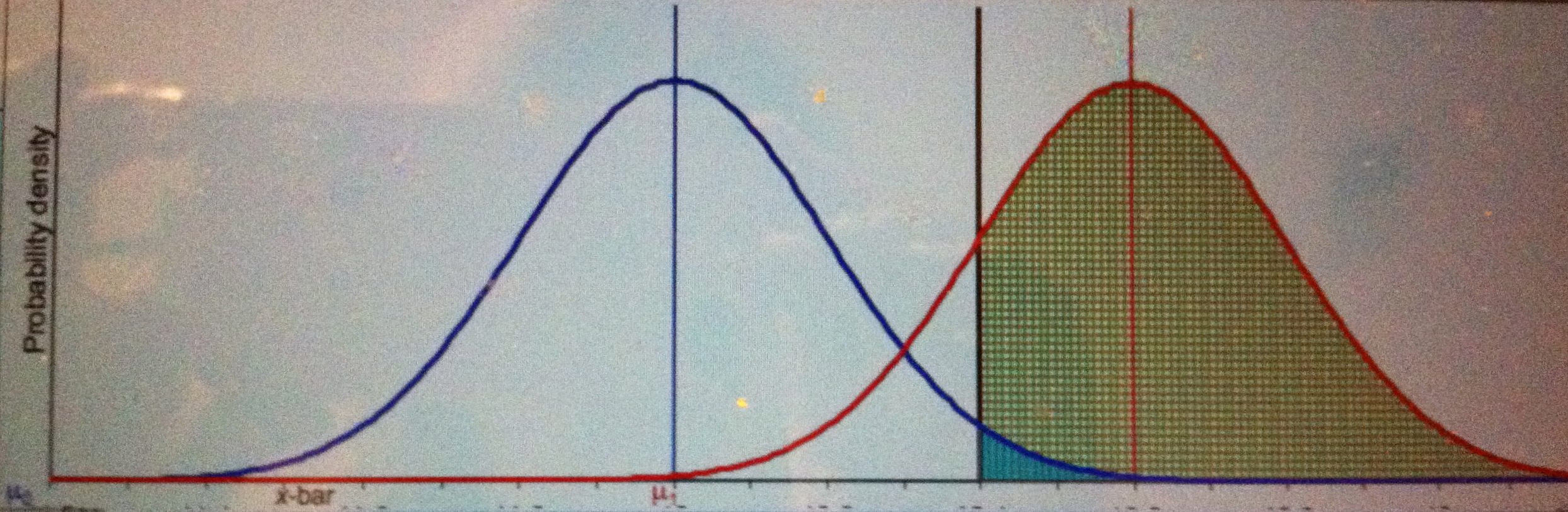
Blue curve is the null, red curve is one possible conjectured alternative: µ = 3. Green area is power, little turquoise area is α.

Note that the evidence our result affords µ > µ’ gets worse and worse as we drag µ further and further to the right, even though in so doing we’re increasing the power.  

As Stephen Senn points out (in my favorite of his guest posts), the alternative against which we set high power is the discrepancy from the null that “we should not like to miss”, delta Δ.  Δ is not the discrepancy we may infer from a significant result (in a test where POW(Δ) = .84), nor one that we believe obtains.

So the correct answer is B.

Does A hold true if we happen to know (based on previous severe tests) that µ <µ’? 

No, but it does allow some legitimate ways to mount complaints based on a significant result from a test with low power to detect a known discrepancy.

It does mean that if M* (the cut-off for a result just statistically significant at level α) is used as an estimate of µ, with no standard error given, although we know independently that µ < M*, then M* is larger than µ. This is a tautology, and crucial information about the unreliability of the estimate is hidden. While it might be said that your observed result, which we’re assuming is M*, “exaggerates” µ, if you were to use it as an estimate, without reporting the SE, it is more correctly describing a misuse of tests, which would direct you to use the lower limit of a confidence interval if you were keen to estimate effect size once finding significance. Why is it highly unkosher for a significance tester? Despite knowing µ < M* (one of the givens of the example), it’s estimated as M*–as if there’s no uncertainty. 

If the study is in a field known to have lots of researcher flexibility, it might legitimately raise the question of whether the researchers cheated, reporting only the one impressive result after trying and trying again, or tampered with the discretionary points of the study to achieve nominal significance. This is a different issue, and doesn’t change my answer. More generally, it’s because the answer is B that the only way to raise the criticism legitimately is to challenge the assumptions of the test.

Why does the criticism arise illegitimately? There are a few reasons. In some circles it’s a direct result of trying to do a Bayesian computation and setting about to compute Pr(µ = µ’|Mo = M*) using POW(µ’)/α as a kind of likelihood ratio in favor of µ’.  Notice that supposing the probability of a type I error goes down as power increases is at odds with the trade-off that we know holds between these error rates. So this immediately indicates a different use of terms. 

[1] This is a modified reblog of an earlier post. 

*Point on language: “to detect alternative µ'” means, “produce a statistically significant result when µ = µ’.” It does not mean we infer µ’. Nor do we know the underlying µ’ after we see the data, obviously. The power of the test to detect µ’ just refers to the probability the test would produce a result that rings the significance alarm, if the data were generated from a world or experiment where µ = µ’.


Categories: blizzard of 26 power puzzles, power, reforming the reformers | 1 Comment

A Blizzard of Power Puzzles Replicate in Meta-Research

.

I often say that the most misunderstood concept in error statistics is power. One week ago, stuck in the blizzard of 2026 in NYC —exciting, if also a bit unnerving, with airports closed for two and a half days and no certainty of when I might fly out—I began collecting the many power howlers I’ve discussed in the past, because some of them are being replicated in todays meta-research about replication failure! Apparently, mistakes about statistical concepts replicate quite reliably—even when statistically significant effects do not. Others I find in medical reports of clinical trials of treatments I’m trying to evaluate in real life! Here’s one variant: A statistically significant result in a clinical trial with fairly high (e.g.,  .8) power to detect an impressive improvement δ’ is taken as good evidence of its impressive improvement δ’. Often the high power of .8 is even used as a (posterior) probability of the hypothesis of improvement being δ’. [0] If these do not immediately strike you as fallacious, compare:

  • If the house is fully ablaze, then very probably the fire alarm goes off.
  • If the fire alarm goes off, then very probably the house is fully ablaze.

The first bullet is saying the fire alarm has high power to detect the house being fully ablaze. It does not mean the converse in the second bullet.

Today’s meta-statistical researchers are keen to point up the consequences of using statistical significance tests, figuring out why they lead to the various replication crises in science, and how they may be more honestly viewed. Yet they too use statistical analyses, and these can reflect philosophical and conceptual standpoints that may replicate the same shortcomings that arise in classic criticisms of significance tests.  A major purpose of my Statistical Inference as Severe Testing: How to Get Beyond the Statistics Wars (2018, CUP) is to clarify basic notions to get beyond what I call “chestnuts” and “howlers” of tests, but these misunderstandings tend to crop up today at the meta-level. When power enters this meta-research, often as a kind of probability of replication, unsurprisingly, the same confusions pop up at the meta-level. But I will not tackle any meta-research in this post. Instead, let’s go back to power howlers that arise in criticisms of tests. I had a blogpost long ago on Ziliac and McCloskey (2008) (Z & M) on power (from Oct. 2011), following a review of their book by Aris Spanos (2008). They write:

“The error of the second kind is the error of accepting the null hypothesis of (say) zero effect when the null is in face false, that is, when (say) such and such a positive effect is true.”

So far so good, keeping in mind that “positive effect” refers to a parameter discrepancy, say δ, not an observed difference.

And the power of a test to detect that such and such a positive effect δ is true is equal to the probability of rejecting the null hypothesis of (say) zero effect when the null is in fact false, and a positive effect as large as δ is present.

Fine. Let this alternative be abbreviated H’(δ):

H’(δ): there is a positive (population) effect at least as large as δ.

Suppose the test rejects the null when it reaches a significance level of .01 (nothing turns on the small value chosen).

(1) The power of the test to detect H’(δ) = Pr(test rejects null at the .01 level| H’(δ) is true).

Say it is 0.85.

According to Z & M:

“[If] the power of a test is high, say, 0.85 or higher, then the scientist can be reasonably confident that at minimum the null hypothesis (of, again, zero effect if that is the null chosen) is false and that therefore his rejection of it is highly probably correct.” (Z & M, 132-3)

But this is not so. They are mistaking (1), defining power, as giving a posterior probability of .85–either to some effect, or specifically to H’(δ)! That is, (1) is being transformed to (1′):

(1’) Pr(H’(δ) is true| test rejects null at .01 level)=.85!

(I am using the symbol for conditional probability “|” all the way through for ease in following the argument, even though, strictly speaking, the error statistician would use “;”, abbreviating “under the assumption that”). Or to put this in other words, they argue:

1. Pr(test rejects the null | H’(δ) is true) = 0.85.

2. Test rejects the null hypothesis.

Therefore, the rejection is probably correct, e.g., the probability H’ is true is 0.85.

Oops. Premises 1 and 2 are true, but the conclusion fallaciously replaces premise 1 with 1′.


High power as high hurdle. As Aris Spanos (2008) points out, “They have it backwards”.  Their reasoning comes from thinking that the higher the power of the test from which statistical significance emerges, the higher the hurdle it has gotten over. Extracting from a Spanos comment on this blog in 2011:

“When [Ziliak and McCloskey] claim that: ‘What is relevant here for the statistical case is that refutations of the null are trivially easy to achieve if power is low enough or the sample size is large enough.’ (Z & M, p. 152), they exhibit [confusion] about the notion of power and its relationship to the sample size; their two instances of ‘easy rejection’ separated by ‘or’ contradict each other! Rejections of the null are not easy to achieve when the power is ‘low enough’. They are more difficult exactly because the test does not have adequate power (generic capacity) to detect discrepancies from the null; that stems from the very definition of power and optimal tests. [Their second claim] is correct for the wrong reason. Rejections are easy to achieve when the sample size n is large enough due to high not low power. This is because the power of a ‘decent’ (consistent) frequentist test increases monotonically with n!” (Spanos 2011) [i]

 Ziliak and McCloskey (2008) tell us: “It is the history of Fisher significance testing. One erects little significancehurdles, six inches tall, and makes a great show of leaping over them, . . . If a test does a good job of uncovering efficacy, then the test has high power and the hurdles are high not low.” (ibid., p. 133) This explains why they suppose high power translates into high hurdles, but it is the opposite. The higher the hurdle required before rejecting the null, the more difficult it is to reject, and the lower the power. High hurdles correspond to insensitive tests, like insensitive fire alarms. It might be that using sensitivityrather than power would make this abundantly clear. We may coin: The high power = high hurdle (for rejecting the null) fallacy. A powerful test does give the null hypothesis a harder time in the sense that its more probable that discrepancies from it are detected. But this makes it easier to infer H1. To infer H1 with severity, H1 needs to be given a hard time. 

Ponder the consequences their construal would have for the required trade-off between type 1 and type 2 error probabilities. (Use the comments to explain what happens.) For a fuller discussion, see this link to Excursion 5 Tour I of SIST (2018). [ii] [iii]

What power howlers have you found? Share them in the comments and I’ll add them to my blizzard. 

Spanos, A. (2008), Review of S. Ziliak and D. McCloskey’s The Cult of Statistical SignificanceErasmus Journal for Philosophy and Economics, volume 1, issue 1: 154-164.

Ziliak, Z. and McCloskey, D. (2008), The Cult of Statistical Significance: How the Standard Error Costs Us Jobs, Justice and Lives, University of Michigan Press.

[0] Some meta-researchers, having brilliently generated a superpopulation of treatments (from which this one is taken as a random sample), and finding these probabilities don’t hold, take this to show p-values exaggerate effects. I’ll come back to that case, which is a bit different from the one in today’s post.

[i] When it comes to raising the power by increasing sample size, Z & M often make true claims, so it’s odd when there’s a switch, as when they say “refutations of the null are trivially easy to achieve if power is low enough or the sample size is large enough”. (Z & M, p. 152) It is clear that “low” is not a typo here either (as I at first assumed), so it’s mysterious. 

[ii] Remember that a power computation is not the probability of data x under some alternative hypothesis, it’s the probability that data fall in the rejection region of a test under some alternative hypothesis. In terms of a test statistic d(X), it is Pr(test statistic d(X) is statistically significant | H’ true), at a given level of significance. So it’s the probability of getting any of the outcomes that would lead to statistical significance at the chosen level, under the assumption that alternative H’ is true. The alternative H’ used to compute power is a point in the alternative region. However, the inference that is made in tests is not to a point hypothesis but to an inequality, e.g., θ > θ’. 

[iii] My rendering of their fallacy above sees it as a type of affirming the consequent. They are right that if inference is by way of a Bayes boost, then affirming the consequent is not a fallacy. A hypothesis H that entails (or renders probable) data x will get a “B-boost” from x, unless its probability is already 1. The trouble erupts when Z & M take an error statistical concept like power, and construe it Bayesianly. Even more confusing, they only do so some of the time.

The next blizzard 26 of power puzzles on this blog is here

Categories: blizzard of 26, power, SIST, statistical significance tests | Tags: , , | 11 Comments

Leisurely Cruise February 2026: power, shpower, positive predictive value

2025-6 Leisurely Cruise

The following is the February stop of our leisurely cruise (meeting 6 from my 2020 Seminar at the LSE). There was a guest speaker, Professor David Hand. Slides and videos are below. Ship StatInfasSt may head back to port or continue for an additional stop or two, if there is interest. Although I often say on this blog that the classical notion of power, as defined by Neyman and Pearson, is one of the most misunderstood notions in stat foundations. I did not know, in writing SIST, just how ingrained those misconceptions would become. I’ll write more on this in my next post. (The following is from SIST pp. 354-356, the pages are provided below)

Shpower and Retrospective Power Analysis

It’s unusual to hear books condemn an approach in a hush-hush sort of way without explaining what’s so bad about it. This is the case with something called post hoc power analysis, practiced by some who live on the outskirts of Power Peninsula. Psst, don’t go there. We hear “there’s a sinister side to statistical power, … I’m referring to post hoc power” (Cumming 2012, pp. 340-1), also called observed power and retrospective (retro) power. I will be calling it shpower analysis. It distorts the logic of ordinary power analysis (from insignificant results). The “post hoc” part comes in because it’s based on the observed results. The trouble is that ordinary power analysis is also post-data. The criticisms are often wrongly taken to reject both.

Shpower evaluates power with respect to the hypothesis that the population effect size (discrepancy) equals the observed effect size, for example, that the parameter μ equals the observed mean. In T+ this would be to set μ = x. Conveniently, their examples use variations on test T+. We may define:

The Shpower of test T+: Pr(X > xα; μ = x)

The thinking, presumably, is that, since we don’t know the value of μ, we might use the observed x to estimate it, and then compute power in the usual way, except substituting the observed value. But a moment’s thought shows the problem – at least for the purpose of using power analysis to interpret insignificant results. Why?

Since alternative μ is set equal to the observed x, and x is given as statistically insignificant, we know we are in Case 1 from Section 5.1: the power can never exceed 0.5. In other words, since  x < xα, the shpower = POW(T+, μ = x) . But power analytic reasoning is all about finding an alternative against which the test has high capability to have rung the significance bell, were that the true parameter value – high power. Shpower is always “slim” (to echo Neyman) against such alternatives. Unsurprisingly, then, shpower analytical reasoning has been roundly criticized in the literature. But the critics think they’re maligning power analytic reasoning.

Now we know the severe tester insists on using attained power Pr(d(X) > d(x0); μ’) to evaluate severity, but when addressing the criticisms of power analysis, we have to stick to ordinary power:[1]

Ordinary power: POW(μ’): Pr(d(X) > cα; μ’)
Shpower (aka post hoc or retro power): Pr(d(X) > cα; μ = x)

An article by Hoenig and Heisey (2001) (“The Abuse of Power”) calls power analysis abusive. Is it? Aris Spanos and I say no (in a 2002 note on them), but the journal declined to publish it [because the deadline for comments had passed]. Since then their slips have spread like kudzu through the literature.

Howlers of Shpower Analysis

Hoenig and Heisey notice that within the class of insignificant results, the more significant the observed x is, the higher the “observed power” against μ = x, until it reaches 0.5 (when x reaches xα and becomes significant). “That’s backwards!” they howl. It is backwards if “observed power” is defined as shpower. Because, if you were to regard higher shpower as indicating better evidence for the null, you’d be saying the more statistically significant the observed difference (between x and μ0), the more the evidence of the absence of a discrepancy from the null hypothesis μ0. That would contradict the logic of tests.

Two fallacies are being committed here. The first we dealt with in discussing Greenland: namely, supposing that a negative result, with high power against μ1, is evidence for the null rather than merely evidence that μ < μ1.The more serious fallacy is that their “observed power” is shpower. Neither Cohen nor Neyman define power analysis this way. It is concluded that power analysis is paradoxical and inconsistent with -value reasoning. You should really only conclude that shpower analytic reasoning is paradoxical. If you’ve redefined a concept and find that a principle that held with the original concept is contradicted, you should suspect your redefinition. It might have other uses, but there is no warrant to discredit the original notion.

The shpower computation is asking: What’s the probability of getting X > xα under μ = x? We still have that the larger the power (against μ = x), the better x indicates that μ < x – as in ordinary power analysis – it’s just that the indication is never more than 0.5. Other papers and even instructional manuals (Ellis 2010) assume shpower as what retrospective power analysis must mean, and ridicule it because “a nonsignificant result will almost always be associated with low statistical power” (p. 60). Not so. I’m afraid that observed power and retrospective power are all used in the literature to mean shpower. What about my use of severity? Severity will replace the cutoff for rejection with the observed value of the test statistic (i.e., Pr(d(X) > d(x0); μ1)), but not the parameter value μ. You might say, we don’t know the value of μ1. True, but that doesn’t stop us from forming power or severity curves and interpreting results accordingly. Let’s leave shpower and consider criticisms of ordinary power analysis. Again, pointing to Hoenig and Heisey’s article (2001) is ubiquitous.

[1] In deciphering existing discussions on ordinary power analysis, we can suppose that d(x0)  happens to be exactly at the cut-off for rejection, in discussing significant results; and just misses the cut-off for discussions on insignificant results in test T+. Then att-power for μ1 equals ordinary power for μ1 .

Reading:

SIST Excursion 5 Tour I (pp. 323-332; 338-344; 346-352),Tour II (pp. 353-6; 361-370), and Farewell Keepsake pp. 436-444

Recommended (if time) What Ever Happened to Bayesian Foundations (Excursion 6 Tour I)


Mayo Memos for Meeting 6:

-Souvenirs Meeting 6: W: The Severity Interpretation of Negative Results (SIN) for Test T+; X: Power and Severity Analysis; Z: Understanding Tribal Warfare

-Selected blogposts on Power

  • 05/08/17: How to tell what’s true about power if you’re practicing within the error-statistical tribe
  • 12/12/17: How to avoid making mountains out of molehills (using power and severity)

There is also a guest speaker: Professor David Hand:
      “Trustworthiness of Statistical Analysis”

_______________________________________________________________________________________________________

Slides & Video Links for Meeting 6:

Slides: Mayo 2nd Draft slides for 25 June (not beautiful)

Video of Meeting #6: (Viewing Videos in full screen mode helps with buffering issues.)
VIDEO LINK:
https://wp.me/abBgTB-mZ

VIDEO LINK to David Hand’s Presentation: https://wp.me/abBgTB-mS
David Hand’s recorded Powerpoint slides: https://wp.me/abBgTB-n4
AUDIO LINK to David Hand’s Presentation & Discussion: https://wp.me/abBgTB-nm

Another link is here.

Please share your thoughts and queries in the comments.

Categories: 2025-2026 Leisurely Cruise, power | Leave a comment

Are We Listening? Part II of “Sennsible significance” Commentary on Senn’s Guest Post

.

This is Part II of my commentary on Stephen Senn’s guest postBe Careful What You Wish For. In this follow-up, I take up two topics:

(1) A terminological point raised in the comments to Part I, and
(2) A broader concern about how a popular reform movement reinforces precisely the mistaken construal Senn warns against.

But first, a question—are we listening? Because what underlies what Senn is saying is subtle, and yet what’s at stake is quite important for today’s statistical controversies. It’s not just a matter of which of four common construals is most apt for the population effect we wish to have high power to detect.[1] As I hear Senn, he’s also flagging a misunderstanding that allows some statistical reformers to (wrongly) dictate what statistical significance testers “wish” for in the first place. Continue reading

Categories: clinical relevance, power, reforming the reformers, S. Senn | 5 Comments

“Sennsible significance” Commentary on Senn’s Guest Post (Part I)

.

Have the points in Stephen Senn’s guest post fully come across?  Responding to comments from diverse directions has given Senn a lot of work, for which I’m very grateful. But I say we should not leave off the topic just yet. I don’t think the core of Senn’s argument has gotten the attention it deserves. So, we’re not done yet.[0]

I will write my commentary in two parts, so please return for Part II. In Part I, I’ll attempt to give an overarching version of Senn’s warning (“Be careful what you wish for”) and  his main recommendation. He will tell me if he disagrees. All quotes are from his post. In Senn’s opening paragraph:

…Even if a hypothesis is rejected and the effect is assumed genuine, it does not mean it is important…many a distinguished commentator on clinical trials has confused the difference you would be happy to find with the difference you would not like to miss. The former is smaller than the latter. For reasons I have explained in this blog [reblogged here], you should use the latter for determining the sample size as part of a conventional power calculation.

Continue reading

Categories: clinical relevance, power, S. Senn | 6 Comments

Stephen Senn (guest post): “Relevant significance? Be careful what you wish for”


.

Stephen Senn

Consultant Statistician
Edinburgh

Relevant significance?

Be careful what you wish for

Despised and Rejected

Scarcely a good word can be had for statistical significance these days. We are admonished (as if we did not know) that just because a null hypothesis has been ‘rejected’ by some statistical test, it does not mean it is not true and thus it does not follow that significance implies a genuine effect of treatment. Continue reading

Categories: clinical relevance, power, S. Senn | 47 Comments

(Guest Post) Stephen Senn: “Delta Force: To what extent is clinical relevance relevant?” (reblog)

Stephen Senn

Senn

Errorstatistics.com has been extremely fortunate to have contributions by leading medical statistician, Stephen Senn, over many years. Recently, he provided me with a new post that I’m about to put up, but as it builds on an earlier post, I’ll reblog that one first. Following his new post, I’ll share some reflections on the issue.

Stephen Senn
Consultant Statistician
Edinburgh, Scotland

Delta Force
To what extent is clinical relevance relevant?

Inspiration
This note has been inspired by a Twitter exchange with respected scientist and famous blogger  David Colquhoun. He queried whether a treatment that had 2/3 of an effect that would be described as clinically relevant could be useful. I was surprised at the question, since I would regard it as being pretty obvious that it could but, on reflection, I realise that things that may seem obvious to some who have worked in drug development may not be obvious to others, and if they are not obvious to others are either in need of a defence or wrong. I don’t think I am wrong and this note is to explain my thinking on the subject. Continue reading

Categories: power, Statistics, Stephen Senn | 2 Comments

A statistically significant result indicates H’ (μ > μ’) when POW(μ’) is low (not the other way round)–but don’t ignore the standard error

.

1. New monsters. One of the bizarre facts of life in the statistics wars is that a method from one school may be criticized on grounds that it conflicts with a conception that is the reverse of what that school intends. How is that even to be deciphered? That was the difficult task I set for myself in writing Statistical Inference as Severe Testing: How to Get Beyond the Statistics Wars (CUP, 2008) [SIST 2018]. I thought I was done, but new monsters keep appearing. In some cases, rather than see how the notion of severity gets us beyond fallacies, misconstruals are taken to criticize severity! So, for example, in the last couple of posts, here and here, I deciphered some of the better known power howlers (discussed in SIST Ex 5 Tour II) I’m linking to all of this tour (in proofs). Continue reading

Categories: power, reforming the reformers, SIST, Statistical Inference as Severe Testing | 16 Comments

Do “underpowered” tests “exaggerate” population effects? (iv)

.

You will often hear that if you reach a just statistically significant result “and the discovery study is underpowered, the observed effects are expected to be inflated” (Ioannidis 2008, p. 64), or “exaggerated” (Gelman and Carlin 2014). This connects to what I’m referring to as the second set of concerns about statistical significance tests, power and magnitude errors. Here, the problem does not revolve around erroneously interpreting power as a posterior probability, as we saw in the fallacy in this post. But there are other points of conflict with the error statistical tester, and much that cries out for clarification — else you will misunderstand the consequences of some of today’s reforms.. Continue reading

Categories: power, reforming the reformers, SIST, Statistical Inference as Severe Testing | 17 Comments

Join me in reforming the “reformers” of statistical significance tests

.

The most surprising discovery about today’s statistics wars is that some who set out shingles as “statistical reformers” themselves are guilty of misdefining some of the basic concepts of error statistical tests—notably power. (See my recent post on power howlers.) A major purpose of my Statistical Inference as Severe Testing: How to Get Beyond the Statistics Wars (2018, CUP) is to clarify basic notions to get beyond what I call “chestnuts” and “howlers” of tests. The only way that disputing tribes can get beyond the statistics wars is by (at least) understanding correctly the central concepts. But these misunderstandings are more common than ever, so I’m asking readers to help. Why are they more common (than before the “new reformers” of the last decade)? I suspect that at least one reason is the popularity of Bayesian variants on tests: if one is looking to find posterior probabilities of hypotheses, then error statistical ingredients may tend to look as if that’s what they supply.  Continue reading

Categories: power, SIST, statistical significance tests | Tags: , , | 2 Comments

S. Senn: The Power of Negative Thinking (guest post)

.


Stephen Senn
Consultant Statistician
Edinburgh, Scotland

Sepsis sceptic

During an exchange on Twitter, Lawrence Lynn drew my attention to a paper by Laffey and Kavanagh[1]. This makes an interesting, useful and very depressing assessment of the situation as regards clinical trials in critical care. The authors make various claims that RCTs in this field are not useful as currently conducted. I don’t agree with the authors’ logic here although, perhaps, surprisingly, I consider that their conclusion might be true. I propose to discuss this here. Continue reading

Categories: power, randomization | 5 Comments

Bonus meeting: Graduate Research Seminar: Current Controversies in Phil Stat: LSE PH 500: 25 June 2020

Ship StatInfasSt

We’re holding a bonus, 6th, meeting of the graduate research seminar PH500 for the Philosophy, Logic & Scientific Method Department at the LSE:

(Remote 10am-12 EST, 15:00 – 17:00 London time; Thursday, June 25)

VI. (June 25) BONUS: Power, shpower, severity, positive predictive value (diagnostic model) & a Continuation of The Statistics Wars and Their Casualties

There will also be a guest speaker: Professor David Hand (Imperial College, London). Here is Professor Hand’s presentation (click on “present” to hear sound)

The main readings are on the blog page for the seminar.


Categories: Graduate Seminar PH500 LSE, power | Leave a comment

(Full) Excerpt. Excursion 5 Tour II: How Not to Corrupt Power (Power Taboos, Retro Power, and Shpower)

.

returned from London…

The concept of a test’s power is still being corrupted in the myriad ways discussed in 5.5, 5.6.  I’m excerpting all of Tour II of Excursion 5, as I did with Tour I (of Statistical Inference as Severe Testing:How to Get Beyond the Statistics Wars 2018, CUP)*. Originally the two Tours comprised just one, but in finalizing corrections, I decided the two together was too long of a slog, and I split it up. Because it was done at the last minute, some of the terms in Tour II rely on their introductions in Tour I.  Here’s how it starts:

5.5 Power Taboos, Retrospective Power, and Shpower

Let’s visit some of the more populous tribes who take issue with power – by which we mean ordinary power – at least its post-data uses. Power Peninsula is often avoided due to various “keep out” warnings and prohibitions, or researchers come during planning, never to return. Why do some people consider it a waste of time, if not totally taboo, to compute power once we know the data? A degree of blame must go to N-P, who emphasized the planning role of power, and only occasionally mentioned its use in determining what gets “confirmed” post-data. After all, it’s good to plan how large a boat we need for a philosophical excursion to the Lands of Overlapping Statistical Tribes, but once we’ve made it, it doesn’t matter that the boat was rather small. Or so the critic of post-data power avers. A crucial disanalogy is that with statistics, we don’t know that we’ve “made it there,” when we arrive at a statistically significant result. The statistical significance alarm goes off, but you are not able to see the underlying discrepancy that generated the alarm you hear. The problem is to make the leap from the perceived alarm to an aspect of a process, deep below the visible ocean, responsible for its having been triggered. Then it is of considerable relevance to exploit information on the capability of your test procedure to result in alarms going off (perhaps with different decibels of loudness), due to varying values of the parameter of interest. There are also objections to power analysis with insignificant results. Continue reading

Categories: fallacy of non-significance, power, Statistical Inference as Severe Testing | Leave a comment

How to avoid making mountains out of molehills (using power and severity)

.

In preparation for a new post that takes up some of the recent battles on reforming or replacing p-values, I reblog an older post on power, one of the most misunderstood and abused notions in statistics. (I add a few “notes on howlers”.)  The power of a test T in relation to a discrepancy from a test hypothesis H0 is the probability T will lead to rejecting H0 when that discrepancy is present. Power is sometimes misappropriated to mean something only distantly related to the probability a test leads to rejection; but I’m getting ahead of myself. This post is on a classic fallacy of rejection. Continue reading

Categories: CIs and tests, Error Statistics, power | 8 Comments

Frequentstein’s Bride: What’s wrong with using (1 – β)/α as a measure of evidence against the null?

Slide1

.

ONE YEAR AGO: …and growing more relevant all the time. Rather than leak any of my new book*, I reblog some earlier posts, even if they’re a bit scruffy. This was first blogged here (with a slightly different title). It’s married to posts on “the P-values overstate the evidence against the null fallacy”, such as this, and is wedded to this one on “How to Tell What’s True About Power if You’re Practicing within the Frequentist Tribe”. 

In their “Comment: A Simple Alternative to p-values,” (on the ASA P-value document), Benjamin and Berger (2016) recommend researchers report a pre-data Rejection Ratio:

It is the probability of rejection when the alternative hypothesis is true, divided by the probability of rejection when the null hypothesis is true, i.e., the ratio of the power of the experiment to the Type I error of the experiment. The rejection ratio has a straightforward interpretation as quantifying the strength of evidence about the alternative hypothesis relative to the null hypothesis conveyed by the experimental result being statistically significant. (Benjamin and Berger 2016, p. 1)

Continue reading

Categories: Bayesian/frequentist, fallacy of rejection, J. Berger, power, S. Senn | 17 Comments

How to tell what’s true about power if you’re practicing within the error-statistical tribe

two_pink_clouds

.

This is a modified reblog of an earlier post, since I keep seeing papers that confuse this.

Suppose you are reading about a result x  that is just statistically significant at level α (i.e., P-value = α) in a one-sided test T+ of the mean of a Normal distribution with n iid samples, and (for simplicity) known σ:   H0: µ ≤  0 against H1: µ >  0. 

I have heard some people say:

A. If the test’s power to detect alternative µ’ is very low, then the just statistically significant x is poor evidence of a discrepancy (from the null) corresponding to µ’.  (i.e., there’s poor evidence that  µ > µ’ ).*See point on language in notes.

They will generally also hold that if POW(µ’) is reasonably high (at least .5), then the inference to µ > µ’ is warranted, or at least not problematic.

I have heard other people say:

B. If the test’s power to detect alternative µ’ is very low, then the just statistically significant x is good evidence of a discrepancy (from the null) corresponding to µ’ (i.e., there’s good evidence that  µ > µ’).

They will generally also hold that if POW(µ’) is reasonably high (at least .5), then the inference to µ > µ’ is unwarranted.

Which is correct, from the perspective of the (error statistical) philosophy, within which power and associated tests are defined? Continue reading

Categories: power, reforming the reformers | 17 Comments

“Nonsignificance Plus High Power Does Not Imply Support for the Null Over the Alternative.”

images-24

Seeing the world through overly rosy glasses

Taboos about power nearly always stem from misuse of power analysis. Sander Greenland (2012) has a paper called “Nonsignificance Plus High Power Does Not Imply Support for the Null Over the Alternative.”  I’m not saying Greenland errs; the error would be made by anyone who interprets power analysis in a manner giving rise to Greenland’s objection. So what’s (ordinary) power analysis?

(I) Listen to Jacob Cohen (1988) introduce Power Analysis

“PROVING THE NULL HYPOTHESIS. Research reports in the literature are frequently flawed by conclusions that state or imply that the null hypothesis is true. For example, following the finding that the difference between two sample means is not statistically significant, instead of properly concluding from this failure to reject the null hypothesis that the data do not warrant the conclusion that the population means differ, the writer concludes, at least implicitly, that there is no difference. The latter conclusion is always strictly invalid, and is functionally invalid as well unless power is high. The high frequency of occurrence of this invalid interpretation can be laid squarely at the doorstep of the general neglect of attention to statistical power in the training of behavioral scientists. Continue reading

Categories: Cohen, Greenland, power, Statistics | 46 Comments

Frequentstein: What’s wrong with (1 – β)/α as a measure of evidence against the null? (ii)

Slide1

.

In their “Comment: A Simple Alternative to p-values,” (on the ASA P-value document), Benjamin and Berger (2016) recommend researchers report a pre-data Rejection Ratio:

It is the probability of rejection when the alternative hypothesis is true, divided by the probability of rejection when the null hypothesis is true, i.e., the ratio of the power of the experiment to the Type I error of the experiment. The rejection ratio has a straightforward interpretation as quantifying the strength of evidence about the alternative hypothesis relative to the null hypothesis conveyed by the experimental result being statistically significant. (Benjamin and Berger 2016, p. 1)

The recommendation is much more fully fleshed out in a 2016 paper by Bayarri, Benjamin, Berger, and Sellke (BBBS 2016): Rejection Odds and Rejection Ratios: A Proposal for Statistical Practice in Testing Hypotheses. Their recommendation is:

…that researchers should report the ‘pre-experimental rejection ratio’ when presenting their experimental design and researchers should report the ‘post-experimental rejection ratio’ (or Bayes factor) when presenting their experimental results. (BBBS 2016, p. 3)….

The (pre-experimental) ‘rejection ratio’ Rpre , the ratio of statistical power to significance threshold (i.e., the ratio of the probability of rejecting under H1 and H0 respectively), is shown to capture the strength of evidence in the experiment for Hover H0. (ibid., p. 2)

But in fact it does no such thing! [See my post from the FUSION conference here.] J. Berger, and his co-authors, will tell you the rejection ratio (and a variety of other measures created over the years) are entirely frequentist because they are created out of frequentist error statistical measures. But a creation built on frequentist measures doesn’t mean the resulting animal captures frequentist error statistical reasoning. It might be a kind of Frequentstein monster! [1] Continue reading

Categories: J. Berger, power, reforming the reformers, S. Senn, Statistical power, Statistics | 36 Comments

When the rejection ratio (1 – β)/α turns evidence on its head, for those practicing in an error-statistical tribe (ii)

imgres-7

.

I’m about to hear Jim Berger give a keynote talk this afternoon at a FUSION conference I’m attending. The conference goal is to link Bayesian, frequentist and fiducial approaches: BFF.  (Program is here. See the blurb below [0]).  April 12 update below*. Berger always has novel and intriguing approaches to testing, so I was especially curious about the new measure.  It’s based on a 2016 paper by Bayarri, Benjamin, Berger, and Sellke (BBBS 2016): Rejection Odds and Rejection Ratios: A Proposal for Statistical Practice in Testing Hypotheses. They recommend:

that researchers should report what we call the ‘pre-experimental rejection ratio’ when presenting their experimental design and researchers should report what we call the ‘post-experimental rejection ratio’ (or Bayes factor) when presenting their experimental results.” (BBBS 2016)….

“The (pre-experimental) ‘rejection ratio’ Rpre , the ratio of statistical power to significance threshold (i.e., the ratio of the probability of rejecting under H1 and H0 respectively), is shown to capture the strength of evidence in the experiment for H1 over H0 .”

If you’re seeking a comparative probabilist measure, the ratio of power/size can look like a likelihood ratio in favor of the alternative. To a practicing member of an error statistical tribe, however, whether along the lines of N, P, or F (Neyman, Pearson or Fisher), things can look topsy turvy. Continue reading

Categories: confidence intervals and tests, power, Statistics | 31 Comments

How to avoid making mountains out of molehills, using power/severity

images

.

A classic fallacy of rejection is taking a statistically significant result as evidence of a discrepancy from a test (or null) hypothesis larger than is warranted. Standard tests do have resources to combat this fallacy, but you won’t see them in textbook formulations. It’s not new statistical method, but new (and correct) interpretations of existing methods, that are needed. One can begin with a companion to the rule in this recent post:

(1) If POW(T+,µ’) is low, then the statistically significant x is a good indication that µ > µ’.

To have the companion rule also in terms of power, let’s suppose that our result is just statistically significant at a level α. (As soon as the observed difference exceeds the cut-off the rule has to be modified). 

Rule (1) was stated in relation to a statistically significant result x (at level α) from a one-sided test T+ of the mean of a Normal distribution with n iid samples, and (for simplicity) known σ:   H0: µ ≤  0 against H1: µ >  0. Here’s the companion:

(2) If POW(T+,µ’) is high, then an α statistically significant x is a good indication that µ < µ’.
(The higher the POW(T+,µ’) is, the better the indication  that µ < µ’.)

That is, if the test’s power to detect alternative µ’ is high, then the statistically significant x is a good indication (or good evidence) that the discrepancy from null is not as large as µ’ (i.e., there’s good evidence that  µ < µ’).

An account of severe testing based on error statistics is always keen to indicate inferences that are not warranted by the data, as well as those that are. Not only might we wish to indicate which discrepancies are poorly warranted, we can give upper bounds to warranted discrepancies by using (2).

POWER: POW(T+,µ’) = POW(Test T+ rejects H0;µ’) = Pr(M > M*; µ’), where M is the sample mean and M* is the cut-off for rejection. (Since it’s continuous, it doesn’t matter if we write > or ≥.)[i]

EXAMPLE. Let σ = 10, n = 100, so (σ/√n) = 1.  Test T+ rejects Hat the .025 level if  M  > 1.96(1).

Find the power against µ = 2.3. To find Pr(M > 1.96; 2.3), get the standard Normal z = (1.96 – 2.3)/1 = -.84. Find the area to the right of -.84 on the standard Normal curve. It is .8. So POW(T+,2.8) = .8.

For simplicity in what follows, let the cut-off, M*, be 2. Let the observed mean M0 just reach the cut-off  2.

The power against alternatives between the null and the cut-off M* will range from α to .5. Power exceeds .5 only once we consider alternatives greater than M*, for these yield negative z values.  Power fact, POW(M* + 1(σ/√n)) = .84.

That is, adding one (σ/ √n) unit to the cut-off M* takes us to an alternative against which the test has power = .84. So, POW(T+, µ = 3) = .84. See this post.

 By (2), the (just) significant result x is decent evidence that µ< 3, because if µ ≥ 3, we’d have observed a more statistically significant result, with probability .84.  The upper .84 confidence limit is 3. The significant result is much better evidence that µ< 4,  the upper .975 confidence limit is 4 (approx.), etc. 

Reporting (2) is typically of importance in cases of highly sensitive tests, but I think it should always accompany a rejection to avoid making mountains out of molehills. (However, in my view, (2) should be custom-tailored to the outcome not the cut-off.) In the case of statistical insignificance, (2) is essentially ordinary power analysis. (In that case, the interest may be to avoid making molehills out of mountains.) Power analysis, applied to insignificant results, is especially of interest with low-powered tests. For example, failing to find a statistically significant increase in some risk may at most rule out (substantively) large risk increases. It might not allow ruling out risks of concern. Naturally, what counts as a risk of concern is a context-dependent consideration, often stipulated in regulatory statutes.

NOTES ON HOWLERS: When researchers set a high power to detect µ’, it is not an indication they regard µ’ as plausible, likely, expected, probable or the like. Yet we often hear people say “if statistical testers set .8 power to detect µ = 2.3 (in test T+), they must regard µ = 2.3 as probable in some sense”. No, in no sense. Another thing you might hear is, “when H0: µ ≤  0 is rejected (at the .025 level), it’s reasonable to infer µ > 2.3″, or “testers are comfortable inferring µ ≥ 2.3”.  No, they are not comfortable, nor should you be. Such an inference would be wrong with probability ~.8. Given M = 2 (or 1.96), you need to subtract to get a lower confidence bound, if the confidence level is not to exceed .5 . For example, µ > .5 is a lower confidence bound at confidence level .93.

Rule (2) also provides a way to distinguish values within a 1-α confidence interval (instead of choosing a given confidence level and then reporting CIs in the dichotomous manner that is now typical).

At present, power analysis is only used to interpret negative results–and there it is often called “retrospective power”, which is a fine term, but it’s often defined as what I call shpower). Again, confidence bounds could be, but they are not now, used to this end [iii].

Severity replaces M* in (2) with the actual result, be it significant or insignificant. 

Looking at power means looking at the best case (just reaching a significance level) or the worst case (just missing it). This is way too coarse; we need to custom tailor results using the observed data. That’s what severity does, but for this post, I wanted to just illuminate the logic.[ii]

One more thing:  

Applying (1) and (2) requires the error probabilities to be actual (approximately correct): Strictly speaking, rules (1) and (2) have a conjunct in their antecedents [iv]: “given the test assumptions are sufficiently well met”. If background knowledge leads you to deny (1) or (2), it indicates you’re denying the reported error probabilities are the actual ones. There’s evidence the test fails an “audit”. That, at any rate, is what I would argue.

————

[i] To state power in terms of P-values: POW(µ’) = Pr(P < p*; µ’) where P < p* corresponds to rejecting the null hypothesis at the given level.

[ii] It must be kept in mind that statistical testing inferences are going to be in the form of µ > µ’ =µ+ δ,  or µ ≤ µ’ =µ+ δ  or the like. They are not to point values! (Not even to the point µ =M0.) Take a look at the alternative H1: µ >  0. It is not a point value. Although we are going beyond inferring the existence of some discrepancy, we still retain inferences in the form of inequalities. 

[iii] That is, upper confidence bounds are too readily viewed as “plausible” bounds, and as values for which the data provide positive evidence. In fact, as soon as you get to an upper bound at confidence levels of around .6, .7, .8, etc. you actually have evidence µ’ < CI-upper. See this post.

[iv] The “antecedent” of a conditional refers to the statement between the “if” and the “then”.

OTHER RELEVANT POSTS ON POWER

Categories: fallacy of rejection, power, Statistics | 20 Comments

Blog at WordPress.com.