
Neyman & Pearson
3.2 N-P Tests: An Episode in Anglo-Polish Collaboration*
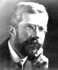
We proceed by setting up a specific hypothesis to test, H0 in Neyman’s and my terminology, the null hypothesis in R. A. Fisher’s . . . in choosing the test, we take into account alternatives to H0 which we believe possible or at any rate consider it most important to be on the look out for . . .Three steps in constructing the test may be defined:
Step 1. We must first specify the set of results . . .
Step 2. We then divide this set by a system of ordered boundaries . . .such that as we pass across one boundary and proceed to the next, we come to a class of results which makes us more and more inclined, on the information available, to reject the hypothesis tested in favour of alternatives which differ from it by increasing amounts.
Step 3. We then, if possible, associate with each contour level the chance that, if H0 is true, a result will occur in random sampling lying beyond that level . . .
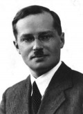
In our first papers [in 1928] we suggested that the likelihood ratio criterion, λ, was a very useful one . . . Thus Step 2 proceeded Step 3. In later papers [1933–1938] we started with a fixed value for the chance, ε, of Step 3 . . . However, although the mathematical procedure may put Step 3 before 2, we cannot put this into operation before we have decided, under Step 2, on the guiding principle to be used in choosing the contour system. That is why I have numbered the steps in this order. (Egon Pearson 1947, p. 173)
In addition to Pearson’s 1947 paper, the museum follows his account in “The Neyman–Pearson Story: 1926–34” (Pearson 1970). The subtitle is “Historical Sidelights on an Episode in Anglo-Polish Collaboration”!
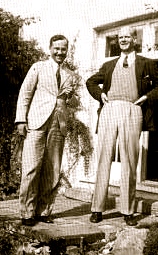
We meet Jerzy Neyman at the point he’s sent to have his work sized up by Karl Pearson at University College in 1925/26. Neyman wasn’t that impressed: Continue reading →


 Excursion 3 Statistical Tests and Scientific Inference


")

