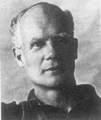
Statistics

Was Janina Hosiasson pulling Harold Jeffreys’ leg?

Posted on October 5, 2013 by Mayo

Hosiasson 1899-1942

The very fact that Jerzy Neyman considers she might have been playing a “mischievous joke” on Harold Jeffreys (concerning probability) is enough to intrigue and impress me (with Hosiasson!). I’ve long been curious about what really happened. Eleonore Stump, a leading medieval philosopher and friend (and one-time colleague), and I pledged to travel to Vilnius to research Hosiasson. I first heard her name from Neyman’s dedication of Lectures and Conferences in Mathematical Statistics and Probability: “To the memory of: Janina Hosiasson, murdered by the Gestapo” along with around 9 other “colleagues and friends lost during World War II.” (He doesn’t mention her husband Lindenbaum, shot alongside her*.) Hosiasson is responsible for Hempel’s Raven Paradox, and I definitely think we should be calling it Hosiasson’s (Raven) Paradox for much of the lost credit to her contributions to Carnapian confirmation theory[i].

But what about this mischievous joke she might have pulled off with Harold Jeffreys? Or did Jeffreys misunderstand what she intended to say about this howler, or? Since it’s a weekend and all of the U.S. monuments and parks are shut down, you might read this snippet and share your speculations…. The following is from Neyman 1952:

“Example 6.—The inclusion of the present example is occasioned by certain statements of Harold Jeffreys (1939, 300) which suggest that, in spite of my  insistence on the phrase, “probability that an object A will possess the  property B,” and in spite of the five foregoing examples, the definition of  probability given above may be misunderstood.  Jeffreys is an important proponent of the subjective theory of probability  designed to measure the “degree of reasonable belief.” His ideas on the  subject are quite radical. He claims (1939, 303) that no consistent theory of probability is possible without the basic notion of degrees of reasonable belief.  His further contention is that proponents of theories of probabilities alternative to his own forget their definitions “before the ink is dry.” In  Jeffreys’ opinion, they use the notion of reasonable belief without ever  noticing that they are using it and, by so doing, contradict the principles  which they have laid down at the outset.

The necessity of any given axiom in a mathematical theory is something  which is subject to proof. … However, Dr. Jeffreys’ contention that the notion of degrees of reasonable  belief and his Axiom 1are necessary for the development of the theory  of probability is not backed by any attempt at proof. Instead, he considers  definitions of probability alternative to his own and attempts to show by  example that, if these definitions are adhered to, the results of their application would be totally unreasonable and unacceptable to anyone. Some  of the examples are striking. On page 300, Jeffreys refers to an article of  mine in which probability is defined exactly as it is in the present volume.  Jeffreys writes:

 The first definition is sometimes called the “classical” one, and is stated in much  modern work, notably that of J. Neyman.

However, Jeffreys does not quote the definition that I use but chooses  to reword it as follows:

If there are n possible alternatives, for m of which p is true, then the probability of  p is defined to be m/n. 

He goes on to say:

The first definition appears at the beginning of De Moivre’s book (Doctrine of  Chances, 1738). It often gives a definite value to a probability; the trouble is that the  value is one that its user immediately rejects. Thus suppose that we are considering  two boxes, one containing one white and one black ball, and the other one white and  two black. A box is to be selected at random and then a ball at random from that box.  What is the probability that the ball will be white? There are five balls, two of which  are white. Therefore, according to the definition, the probability is 2/5. But most  statistical writers, including, I think, most of those that professedly accept the definition, would give (1/2)•(1/2) + (1/2)•(1/3) = 5/12. This follows at once on the present theory,  the terms representing two applications of the product rule to give the probability of  drawing each of the two white balls. These are then added by the addition rule. But  the proposition cannot be expressed as the disjunction of five alternatives out of twelve.  My attention was called to this point by Miss J. Hosiasson. 

The solution, 2/5, suggested by Jeffreys as the result of an allegedly  strict application of my definition of probability is obviously wrong. The  mistake seems to be due to Jeffreys’ apparently harmless rewording of the  definition. If we adhere to the original wording (p. 4) and, in particular, to the  phrase “probability of an object A having the property B,” then, prior to attempting a solution, we would probably ask ourselves the questions:  ”What are the ‘objects A’ in this particular case?” and “What is the ’property B,’ the probability of which it is desired to compute?” Once  these questions have been asked, the answer to them usually follows and  determines the solution.

In the particular example of Dr. Jeffreys, the objects A are obviously  not balls, but pairs of random selections, the first of a box and the second  of a ball. If we like to state the problem without dangerous abbreviations,  the probability sought is that of a pair of selections ending with a white  ball. All the conditions of there being two boxes, the first with two balls  only and the second with three, etc., must be interpreted as picturesque  descriptions of the F.P.S. of pairs of selections. The elements of this set  fall into four categories, conveniently described by pairs of symbols (1,w), (1,b), (2,w), (2,b), so that, for example, (2,w) stands for a pair of  selections in which the second box was selected in the first instance, and  then this was followed by the selection of the white ball. Denote by n1,w, n1,b, n2,w, and n2,b the (unknown) numbers of the elements of the F.P.S. belonging to each of the above categories, and by n their sum. Then the probability sought is “(Neyman 1952, 10-11).

Then there are the detailed computations from which Neyman gets the right answer (entered 10/9/13):

P{w|pair of selections} = (n1,w + n2,w)/n.

The conditions of the problem imply

P{1|pair of selections} = (n1,w + n1,b)/n = ½,

P{2|pair of selections} = (n2,w + n2,b)/n = ½,

P{w| pair of selections beginning with box No. 1} = n1,w/(n1,w + n1,b) = ½,

P{w| pair of selections beginning with box No. 2} = n2,w/(n2,w + n2,b) = 1/3.

It follows

n1,w = 1/2(n1,w + n1,b) = n/4,

n2,w = 1/3(n2,w + n2,b) = n/6,

P{w|pair of selections} = 5/12.

The method of computing probability used here is a direct enumeration  of elements of the F.P.S. For this reason it is called the “direct method.”  As we can see from this particular example, the direct method is occasionally cumbersome and the correct solution is more easily reached through  the application of certain theorems basic in the theory of probability. These theorems, the addition theorem and the multiplication theorem, are very  easy to apply, with the result that students frequently manage to learn the  machinery of application without understanding the theorems. To check  whether or not a student does understand the theorems, it is advisable to  ask him to solve problems by the direct method. If he cannot, then he  does not understand what he is doing.

Checks of this kind were part of the regular program of instruction in  Warsaw where Miss Hosiasson was one of my assistants. Miss Hosiasson  was a very talented lady who has written several interesting contributions  to the theory of probability. One of these papers deals specifically with  various misunderstandings which, under the high sounding name of paradoxes, still litter the scientific books and journals. Most of these paradoxes originate from lack of precision in stating the conditions of the  problems studied. In these circumstances, it is most unlikely that Miss  Hosiasson could fail in the application of the direct method to a simple  problem like the one described by Dr. Jeffreys. On the other hand, I can  well imagine Miss Hosiasson making a somewhat mischievous joke. 

Some of the paradoxes solved by Miss Hosiasson are quite amusing…….”  (Neyman 1952, 10-13)

What think you? I will offer a first speculation in a comment.

The entire book Neyman (1952) may be found here, in plain text, here.

*June, 2017: I read somewhere today that her husband was killed in 41, so before she was, but all refs I know are sketchy.

[i]Of course there are many good, recent sources on the philosophy and history of Carnap, some of which mention her, but obviously do not touch on this matter. I read that Hosiasson was trying to build a Carnapian-style inductive logic setting out axioms (which to my knowledge Carnap never did). That was what some of my fledgling graduate school attempts had tried, but the axioms always seemed to admit counterexamples (if non-trivial). So much for the purely syntactic approach. But I wish I’d known of her attempts back then, and especially her treatment of paradoxes of confirmation. {I’m sometimes tempted to give a logic for severity, but I fight the temptation.)

REFERENCES

Hosiasson, J. (1931) Why do we prefer probabilities relative to many data? Mind 40 (157): 23-36 (1931)

Hosiasson-Lindenbaum, J. (1940) On confirmation Journal of Symbolic Logic 5 (4): 133-148 (1940)

Hosiasson, J. (1941) Induction et analogie: Comparaison de leur fondement Mind 50 (200): 351-365 (1941)

Hosiasson-Lindenbaum, J. (1948) Theoretical Aspects of the Advancement of Knowledge Synthese 7 (4/5):253 – 261 (1948)

Jeffreys, H. (1939) Theory of Probability (1st ed.). Oxford: The Clarendon Press

Neyman, J. (1952) Lectures and Conferences in Mathematical Statistics and Probability. Graduate School, U.S. Dept. of Agriculture

Categories: Hosiasson, phil/history of stat, Statistics | Tags: Jerzy Neyman, Neyman | 22 Comments

Highly probable vs highly probed: Bayesian/ error statistical differences

Posted on September 29, 2013 by Mayo

A reader asks: “Can you tell me about disagreements on numbers between a severity assessment within error statistics, and a Bayesian assessment of posterior probabilities?” Sure.

There are differences between Bayesian posterior probabilities and formal error statistical measures, as well as between the latter and a severity (SEV) assessment, which differs from the standard type 1 and 2 error probabilities, p-values, and confidence levels—despite the numerical relationships. Here are some random thoughts that will hopefully be relevant for both types of differences. (Please search this blog for specifics.)

1. The most noteworthy difference is that error statistical inference makes use of outcomes other than the one observed, even after the data are available: there’s no other way to ask things like, how often would you find 1 nominally statistically significant difference in a hunting expedition over k or more factors? Or to distinguish optional stopping with sequential trials from fixed sample size experiments. Here’s a quote I came across just yesterday:

“[S]topping ‘when the data looks good’ can be a serious error when combined with frequentist measures of evidence. For instance, if one used the stopping rule [above]…but analyzed the data as if a fixed sample had been taken, one could guarantee arbitrarily strong frequentist ‘significance’ against H₀.” (Berger and Wolpert, 1988, 77).

The worry about being guaranteed to erroneously exclude the true parameter value here is an error statistical affliction that the Bayesian is spared (even though I don’t think they can be too happy about it, especially when HPD intervals are assured of excluding the true parameter value.) See this post for an amusing note; Mayo and Kruse (2001) below; and, if interested, search the (strong) likelihood principle, and Birnbaum.

2. Highly probable vs. highly probed. SEV doesn’t obey the probability calculus: for any test T and outcome x, the severity for both H and ~H might be horribly low. Moreover, an error statistical analysis is not in the business of probabilifying hypotheses but evaluating and controlling the capabilities of methods to discern inferential flaws (problems with linking statistical and scientific claims, problems of interpreting statistical tests and estimates, and problems of underlying model assumptions). This is the basis for applying what may be called the Severity principle. Continue reading →

Categories: Bayesian/frequentist, Error Statistics, P-values, Philosophy of Statistics, Statistics, Stephen Senn, strong likelihood principle | 41 Comments

Blog Contents: August 2013

Posted on September 26, 2013 by Mayo

August 2013
(8/1) Blogging (flogging?) the SLP: Response to Reply- Xi’an Robert
(8/5) At the JSM: 2013 International Year of Statistics
(8/6) What did Nate Silver just say? Blogging the JSM
(8/9) 11^th bullet, multiple choice question, and last thoughts on the JSM
(8/11) E.S. Pearson: “Ideas came into my head as I sat on a gate overlooking an experimental blackcurrant plot”
(8/13) Blogging E.S. Pearson’s Statistical Philosophy
(8/15) A. Spanos: Egon Pearson’s Neglected Contributions to Statistics
(8/17) Gandenberger: How to Do Philosophy That Matters (guest post)
(8/21) Blog contents: July, 2013
(8/22) PhilStock: Flash Freeze
(8/22) A critical look at “critical thinking”: deduction and induction
(8/28) Is being lonely unnatural for slim particles? A statistical argument
(8/31) Overheard at the comedy hour at the Bayesian retreat-2 years on

Categories: Announcement, Statistics | Leave a comment

Statistical Theater of the Absurd: “Stat on a Hot Tin Roof”

Posted on September 22, 2013 by Mayo

Memory lane: Did you ever consider how some of the colorful exchanges among better-known names in statistical foundations could be the basis for high literary drama in the form of one-act plays (even if appreciated by only 3-7 people in the world)? (Think of the expressionist exchange between Bohr and Heisenberg in Michael Frayn’s play Copenhagen, except here there would be no attempt at all to popularize—only published quotes and closely remembered conversations would be included, with no attempt to create a “story line”.) Somehow I didn’t think so. But rereading some of Savage’s high-flown praise of Birnbaum’s “breakthrough” argument (for the Likelihood Principle) today, I was swept into a “(statistical) theater of the absurd” mindset.

The first one came to me in autumn 2008 while I was giving a series of seminars on philosophy of statistics at the LSE. Modeled on a disappointing (to me) performance of The Woman in Black, “A Funny Thing Happened at the [1959] Savage Forum” relates Savage’s horror at George Barnard’s announcement of having rejected the Likelihood Principle!

The current piece taking shape also features George Barnard and since tomorrow (9/23) is his birthday, I’m digging it out of “rejected posts”. It recalls our first meeting in London in 1986. I’d sent him a draft of my paper “Why Pearson Rejected the Neyman-Pearson Theory of Statistics” (later adapted as chapter 11 of EGEK) to see whether I’d gotten Pearson right. He’d traveled quite a ways, from Colchester, I think. It was June and hot, and we were up on some kind of a semi-enclosed rooftop. Barnard was sitting across from me looking rather bemused.

The curtain opens with Barnard and Mayo on the roof, lit by a spot mid-stage. He’s drinking (hot) tea; she, a Diet Coke. The dialogue (is what I recall from the time[i]):

Barnard: I read your paper. I think it is quite good. Did you know that it was I who told Fisher that Neyman-Pearson statistics had turned his significance tests into little more than acceptance procedures?

Mayo: Thank you so much for reading my paper. I recall a reference to you in Pearson’s response to Fisher, but I didn’t know the full extent.

Barnard: I was the one who told Fisher that Neyman was largely to blame. He shouldn’t be too hard on Egon. His statistical philosophy, you are aware, was different from Neyman’s. Continue reading →

Categories: Barnard, phil/history of stat, rejected post, Statistics | Tags: Fisher, George Bernard, Likelihood Principle, Neyman, Pearson | 6 Comments

“When Bayesian Inference Shatters” Owhadi and Scovel (guest post)

Posted on September 14, 2013 by Mayo

I’m extremely grateful to Drs. Owhadi and Scovel for replying to my request for “a plain Jane” explication of their interesting paper, “When Bayesian Inference Shatters”, and especially for permission to post it. If readers want to ponder the paper awhile and send me comments for guest posts or “U-PHILS*” (by OCT 15), let me know. Feel free to comment as usual in the mean time.

—————————————-

Houman Owhadi
Professor of Applied and Computational Mathematics and Control and Dynamical Systems, Computing + Mathematical Sciences,
California Institute of Technology, USA

Clint Scovel
Senior Scientist,

Computing + Mathematical Sciences,
California Institute of Technology, USA

“When Bayesian Inference Shatters: A plain Jane explanation”

This is an attempt at a “plain Jane” presentation of the results discussed in the recent arxiv paper “When Bayesian Inference Shatters” located at http://arxiv.org/abs/1308.6306 with the following abstract:

“With the advent of high-performance computing, Bayesian methods are increasingly popular tools for the quantification of uncertainty throughout science and industry. Since these methods impact the making of sometimes critical decisions in increasingly complicated contexts, the sensitivity of their posterior conclusions with respect to the underlying models and prior beliefs is becoming a pressing question. We report new results suggesting that, although Bayesian methods are robust when the number of possible outcomes is finite or when only a finite number of marginals of the data-generating distribution are unknown, they are generically brittle when applied to continuous systems with finite information on the data-generating distribution. This brittleness persists beyond the discretization of continuous systems and suggests that Bayesian inference is generically ill-posed in the sense of Hadamard when applied to such systems: if closeness is defined in terms of the total variation metric or the matching of a finite system of moments, then (1) two practitioners who use arbitrarily close models and observe the same (possibly arbitrarily large amount of) data may reach diametrically opposite conclusions; and (2) any given prior and model can be slightly perturbed to achieve any desired posterior conclusions.”

Now, it is already known from classical Robust Bayesian Inference that Bayesian Inference has some robustness if the random outcomes live in a finite space or if the class of priors considered is finite-dimensional (i.e. what you know is infinite and what you do not know is finite). What we have shown is that if the random outcomes live in an approximation of a continuous space (for instance, when they are decimal numbers given to finite precision) and your class of priors is finite co-dimensional (i.e. what you know is finite and what you do not know may be infinite) then, if the data is observed at a fine enough resolution, the range of posterior values is the deterministic range of the quantity of interest, irrespective of the size of the data. Continue reading →

Categories: Bayesian/frequentist, Statistics | 40 Comments

(Part 2) Peircean Induction and the Error-Correcting Thesis

Posted on September 10, 2013 by Mayo

C. S. Peirce
9/10/1839 – 4/19/1914

Continuation of “Peircean Induction and the Error-Correcting Thesis”

Deborah G. Mayo
Transactions of the Charles S. Peirce Society: A Quarterly Journal in American Philosophy, Volume 41, Number 2, 2005, pp. 299-319

Part 1 is here.

There are two other points of confusion in critical discussions of the SCT, that we may note here:

I. The SCT and the Requirements of Randomization and Predesignation

The concern with “the trustworthiness of the proceeding” for Peirce like the concern with error probabilities (e.g., significance levels) for error statisticians generally, is directly tied to their view that inductive method should closely link inferences to the methods of data collection as well as to how the hypothesis came to be formulated or chosen for testing.

This account of the rationale of induction is distinguished from others in that it has as its consequences two rules of inductive inference which are very frequently violated (1.95) namely, that the sample be (approximately) random and that the property being tested not be determined by the particular sample x— i.e., predesignation.

The picture of Peircean induction that one finds in critics of the SCT disregards these crucial requirements for induction: Neither enumerative induction nor H-D testing, as ordinarily conceived, requires such rules. Statistical significance testing, however, clearly does.

Suppose, for example that researchers wishing to demonstrate the benefits of HRT search the data for factors on which treated women fare much better than untreated, and finding one such factor they proceed to test the null hypothesis:

H₀: there is no improvement in factor F (e.g. memory) among women treated with HRT.

Having selected this factor for testing solely because it is a factor on which treated women show impressive improvement, it is not surprising that this null hypothesis is rejected and the results taken to show a genuine improvement in the population. However, when the null hypothesis is tested on the same data that led it to be chosen for testing, it is well known, a spurious impression of a genuine effect easily results. Suppose, for example, that 20 factors are examined for impressive-looking improvements among HRT-treated women, and the one difference that appears large enough to test turns out to be significant at the 0.05 level. The actual significance level—the actual probability of reporting a statistically significant effect when in fact the null hypothesis is true—is not 5% but approximately 64% (Mayo 1996, Mayo and Kruse 2001, Mayo and Cox 2006). To infer the denial of H₀, and infer there is evidence that HRT improves memory, is to make an inference with low severity (approximately 0.36).

II Understanding the “long-run error correcting” metaphor

Discussions of Peircean ‘self-correction’ often confuse two interpretations of the ‘long-run’ error correcting metaphor, even in the case of quantitative induction: (a) Asymptotic self-correction (as n approaches ∞): In this construal, it is imagined that one has a sample, say of size n=10, and it is supposed that the SCT assures us that as the sample size increases toward infinity, one gets better and better estimates of some feature of the population, say the mean. Although this may be true, provided assumptions of a statistical model (e.g., the Binomial) are met, it is not the sense intended in significance-test reasoning nor, I maintain, in Peirce’s SCT. Peirce’s idea, instead, gives needed insight for understanding the relevance of ‘long-run’ error probabilities of significance tests to assess the reliability of an inductive inference from a specific set of data, (b) Error probabilities of a test: In this construal, one has a sample of size n, say 10, and imagines hypothetical replications of the experiment—each with samples of 10. Each sample of 10 gives a single value of the test statistic d(X), but one can consider the distribution of values that would occur in hypothetical repetitions (of the given type of sampling). The probability distribution of d(X) is called the sampling distribution, and the correct calculation of the significance level is an example of how tests appeal to this distribution: Thanks to the relationship between the observed d(x) and the sampling distribution of d(X), the former can be used to reliably probe the correctness of statistical hypotheses (about the procedure) that generated the particular 10-fold sample. That is what the SCT is asserting.

It may help to consider a very informal example. Suppose that weight gain is measured by 10 well-calibrated and stable methods, possibly using several measuring instruments and the results show negligible change over a test period of interest. This may be regarded as grounds for inferring that the individual’s weight gain is negligible within limits set by the sensitivity of the scales. Why? While it is true that by averaging more and more weight measurements, i.e., an eleventh, twelfth, etc., one would get asymptotically close to the true weight, that is not the rationale for the particular inference. The rationale is rather that the error probabilistic properties of the weighing procedure (the probability of ten-fold weighings erroneously failing to show weight change) inform one of the correct weight in the case at hand, e.g., that a 0 observed weight increase passes the “no-weight gain” hypothesis with high severity. Continue reading →

Categories: Bayesian/frequentist, C.S. Peirce, Error Statistics, Statistics | 5 Comments

Peircean Induction and the Error-Correcting Thesis (Part I)

Posted on September 10, 2013 by Mayo

C. S. Peirce: 10 Sept, 1839-19 April, 1914

Today is C.S. Peirce’s birthday. I hadn’t blogged him before, but he’s one of my all time heroes. You should read him: he’s a treasure chest on essentially any topic. I’ll blog the main sections of a (2005) paper over the next few days. It’s written for a very general philosophical audience; the statistical parts are pretty informal. Happy birthday Peirce.

Peircean Induction and the Error-Correcting Thesis
Deborah G. Mayo
Transactions of the Charles S. Peirce Society: A Quarterly Journal in American Philosophy, Volume 41, Number 2, 2005, pp. 299-319

Peirce’s philosophy of inductive inference in science is based on the idea that what permits us to make progress in science, what allows our knowledge to grow, is the fact that science uses methods that are self-correcting or error-correcting:

Induction is the experimental testing of a theory. The justification of it is that, although the conclusion at any stage of the investigation may be more or less erroneous, yet the further application of the same method must correct the error. (5.145)

Inductive methods—understood as methods of experimental testing—are justified to the extent that they are error-correcting methods. We may call this Peirce’s error-correcting or self-correcting thesis (SCT):

Self-Correcting Thesis SCT: methods for inductive inference in science are error correcting; the justification for inductive methods of experimental testing in science is that they are self-correcting.

Peirce’s SCT has been a source of fascination and frustration. By and large, critics and followers alike have denied that Peirce can sustain his SCT as a way to justify scientific induction: “No part of Peirce’s philosophy of science has been more severely criticized, even by his most sympathetic commentators, than this attempted validation of inductive methodology on the basis of its purported self-correctiveness” (Rescher 1978, p. 20).

In this paper I shall revisit the Peircean SCT: properly interpreted, I will argue, Peirce’s SCT not only serves its intended purpose, it also provides the basis for justifying (frequentist) statistical methods in science. While on the one hand, contemporary statistical methods increase the mathematical rigor and generality of Peirce’s SCT, on the other, Peirce provides something current statistical methodology lacks: an account of inductive inference and a philosophy of experiment that links the justification for statistical tests to a more general rationale for scientific induction. Combining the mathematical contributions of modern statistics with the inductive philosophy of Peirce, sets the stage for developing an adequate justification for contemporary inductive statistical methodology.

2. Probabilities are assigned to procedures not hypotheses

Peirce’s philosophy of experimental testing shares a number of key features with the contemporary (Neyman and Pearson) Statistical Theory: statistical methods provide, not means for assigning degrees of probability, evidential support, or confirmation to hypotheses, but procedures for testing (and estimation), whose rationale is their predesignated high frequencies of leading to correct results in some hypothetical long-run. A Neyman and Pearson (NP) statistical test, for example, instructs us “To decide whether a hypothesis, H, of a given type be rejected or not, calculate a specified character, x₀, of the observed facts; if x> x₀reject H; if x< x₀ accept H.” Although the outputs of N-P tests do not assign hypotheses degrees of probability, “it may often be proved that if we behave according to such a rule … we shall reject H when it is true not more, say, than once in a hundred times, and in addition we may have evidence that we shall reject H sufficiently often when it is false” (Neyman and Pearson, 1933, p.142).[i]

The relative frequencies of erroneous rejections and erroneous acceptances in an actual or hypothetical long run sequence of applications of tests are error probabilities; we may call the statistical tools based on error probabilities, error statistical tools. In describing his theory of inference, Peirce could be describing that of the error-statistician:

The theory here proposed does not assign any probability to the inductive or hypothetic conclusion, in the sense of undertaking to say how frequently that conclusion would be found true. It does not propose to look through all the possible universes, and say in what proportion of them a certain uniformity occurs; such a proceeding, were it possible, would be quite idle. The theory here presented only says how frequently, in this universe, the special form of induction or hypothesis would lead us right. The probability given by this theory is in every way different—in meaning, numerical value, and form—from that of those who would apply to ampliative inference the doctrine of inverse chances. (2.748)

The doctrine of “inverse chances” alludes to assigning (posterior) probabilities in hypotheses by applying the definition of conditional probability (Bayes’s theorem)—a computation requires starting out with a (prior or “antecedent”) probability assignment to an exhaustive set of hypotheses:

If these antecedent probabilities were solid statistical facts, like those upon which the insurance business rests, the ordinary precepts and practice [of inverse probability] would be sound. But they are not and cannot be statistical facts. What is the antecedent probability that matter should be composed of atoms? Can we take statistics of a multitude of different universes? (2.777)

For Peircean induction, as in the N-P testing model, the conclusion or inference concerns a hypothesis that either is or is not true in this one universe; thus, assigning a frequentist probability to a particular conclusion, other than the trivial ones of 1 or 0, for Peirce, makes sense only “if universes were as plentiful as blackberries” (2.684). Thus the Bayesian inverse probability calculation seems forced to rely on subjective probabilities for computing inverse inferences, but “subjective probabilities” Peirce charges “express nothing but the conformity of a new suggestion to our prepossessions, and these are the source of most of the errors into which man falls, and of all the worse of them” (2.777).

Hearing Pierce contrast his view of induction with the more popular Bayesian account of his day (the Conceptualists), one could be listening to an error statistician arguing against the contemporary Bayesian (subjective or other)—with one important difference. Today’s error statistician seems to grant too readily that the only justification for N-P test rules is their ability to ensure we will rarely take erroneous actions with respect to hypotheses in the long run of applications. This so called inductive behavior rationale seems to supply no adequate answer to the question of what is learned in any particular application about the process underlying the data. Peirce, by contrast, was very clear that what is really wanted in inductive inference in science is the ability to control error probabilities of test procedures, i.e., “the trustworthiness of the proceeding”. Moreover it is only by a faulty analogy with deductive inference, Peirce explains, that many suppose that inductive (synthetic) inference should supply a probability to the conclusion: “… in the case of analytic inference we know the probability of our conclusion (if the premises are true), but in the case of synthetic inferences we only know the degree of trustworthiness of our proceeding (“The Probability of Induction” 2.693).

Knowing the “trustworthiness of our inductive proceeding”, I will argue, enables determining the test’s probative capacity, how reliably it detects errors, and the severity of the test a hypothesis withstands. Deliberately making use of known flaws and fallacies in reasoning with limited and uncertain data, tests may be constructed that are highly trustworthy probes in detecting and discriminating errors in particular cases. This, in turn, enables inferring which inferences about the process giving rise to the data are and are not warranted: an inductive inference to hypothesis H is warranted to the extent that with high probability the test would have detected a specific flaw or departure from what H asserts, and yet it did not.

3. So why is justifying Peirce’s SCT thought to be so problematic?

You can read Section 3 here. (it’s not necessary for understanding the rest).

4. Peircean induction as severe testing

… [I]nduction, for Peirce, is a matter of subjecting hypotheses to “the test of experiment” (7.182).

The process of testing it will consist, not in examining the facts, in order to see how well they accord with the hypothesis, but on the contrary in examining such of the probable consequences of the hypothesis … which would be very unlikely or surprising in case the hypothesis were not true. (7.231)

When, however, we find that prediction after prediction, notwithstanding a preference for putting the most unlikely ones to the test, is verified by experiment,…we begin to accord to the hypothesis a standing among scientific results.

This sort of inference it is, from experiments testing predictions based on a hypothesis, that is alone properly entitled to be called induction. (7.206)

While these and other passages are redolent of Popper, Peirce differs from Popper in crucial ways. Peirce, unlike Popper, is primarily interested not in falsifying claims but in the positive pieces of information provided by tests, with “the corrections called for by the experiment” and with the hypotheses, modified or not, that manage to pass severe tests. For Popper, even if a hypothesis is highly corroborated (by his lights), he regards this as at most a report of the hypothesis’ past performance and denies it affords positive evidence for its correctness or reliability. Further, Popper denies that he could vouch for the reliability of the method he recommends as “most rational”—conjecture and refutation. Indeed, Popper’s requirements for a highly corroborated hypothesis are not sufficient for ensuring severity in Peirce’s sense (Mayo 1996, 2003, 2005). Where Popper recoils from even speaking of warranted inductions, Peirce conceives of a proper inductive inference as what had passed a severe test—one which would, with high probability, have detected an error if present.

In Peirce’s inductive philosophy, we have evidence for inductively inferring a claim or hypothesis H when not only does H “accord with” the data x; but also, so good an accordance would very probably not have resulted, were H not true. In other words, we may inductively infer H when it has withstood a test of experiment that it would not have withstood, or withstood so well, were H not true (or were a specific flaw present). This can be encapsulated in the following severity requirement for an experimental test procedure, ET, and data set x.

Hypothesis H passes a severe test with x iff (firstly) x accords with H and (secondly) the experimental test procedure ET would, with very high probability, have signaled the presence of an error were there a discordancy between what H asserts and what is correct (i.e., were H false).

The test would “have signaled an error” by having produced results less accordant with H than what the test yielded. Thus, we may inductively infer H when (and only when) H has withstood a test with high error detecting capacity, the higher this probative capacity, the more severely H has passed. What is assessed (quantitatively or qualitatively) is not the amount of support for H but the probative capacity of the test of experiment ET (with regard to those errors that an inference to H is declaring to be absent)……….

You can read the rest of Section 4 here.

5. The path from qualitative to quantitative induction

In my understanding of Peircean induction, the difference between qualitative and quantitative induction is really a matter of degree, according to whether their trustworthiness or severity is quantitatively or only qualitatively ascertainable. This reading not only neatly organizes Peirce’s typologies of the various types of induction, it underwrites the manner in which, within a given classification, Peirce further subdivides inductions by their “strength”.

(I) First-Order, Rudimentary or Crude Induction

Consider Peirce’s First Order of induction: the lowest, most rudimentary form that he dubs, the “pooh-pooh argument”. It is essentially an argument from ignorance: Lacking evidence for the falsity of some hypothesis or claim H, provisionally adopt H. In this very weakest sort of induction, crude induction, the most that can be said is that a hypothesis would eventually be falsified if false. (It may correct itself—but with a bang!) It “is as weak an inference as any that I would not positively condemn” (8.237). While uneliminable in ordinary life, Peirce denies that rudimentary induction is to be included as scientific induction. Without some reason to think evidence of H‘s falsity would probably have been detected, were H false, finding no evidence against H is poor inductive evidence for H. H has passed only a highly unreliable error probe. Continue reading →

Categories: Bayesian/frequentist, C.S. Peirce, Error Statistics, Statistics | 6 Comments

Stephen Senn: Open Season (guest post)

Posted on September 5, 2013 by Mayo

Stephen Senn
Head, Methodology and Statistics Group,
Competence Center for Methodology and Statistics (CCMS),
Luxembourg

“Open Season”

The recent joint statement(1) by the Pharmaceutical Research and Manufacturers of America (PhRMA) and the European Federation of Pharmaceutical Industries and Associations(EFPIA) represents a further step in what has been a slow journey towards (one assumes) will be the achieved goal of sharing clinical trial data. In my inaugural lecture of 1997 at University College London I called for all pharmaceutical companies to develop a policy for sharing trial results and I have repeated this in many places since(2-5). Thus I can hardly complain if what I have been calling for for over 15 years is now close to being achieved.

However, I have now recently been thinking about it again and it seems to me that there are some problems that need to be addressed. One is the issue of patient confidentiality. Ideally, covariate information should be exploitable as such often increases the precision of inferences and also the utility of decisions based upon them since they (potentially) increase the possibility of personalising medical interventions. However, providing patient-level data increases the risk of breaching confidentiality. This is a complicated and difficult issue about which, however, I have nothing useful to say. Instead I want to consider another matter. What will be the influence on the quality of the inferences we make of enabling many subsequent researchers to analyse the same data?

One of the reasons that many researchers have called for all trials to be published is that trials that are missing tend to be different from those that are present. Thus there is a bias in summarising evidence from published trial only and it can be a difficult task with no guarantee of success to identify those that have not been published. This is a wider reflection of the problem of missing data within trials. Such data have long worried trialists and the Food and Drug Administration (FDA) itself has commissioned a report on the subject from leading experts(6). On the European side the Committee for Medicinal Products for Human Use (CHMP) has a guideline dealing with it(7).

However, the problem is really a particular example of data filtering and it also applies to statistical analysis. If the analyses that are present have been selected from a wider set, then there is a danger that they do not provide an honest reflection of the message that is in the data. This problem is known as that of multiplicity and there is a huge literature dealing with it, including regulatory guidance documents(8, 9).

Within drug regulation this is dealt with by having pre-specified analyses. The broad outlines of these are usually established in the trial protocol and the approach is then specified in some detail in the statistical analysis plan which is required to be finalised before un-blinding of the data. The strategies used to control for multiplicity will involve some combination of defining a significance testing route (an order in which test must be performed and associated decision rules) and reduction of the required level of significance to detect an event.

I am not a great fan of these manoeuvres, which can be extremely complex. One of my objections is that it is effectively assumed that the researchers who chose them are mandated to circumscribe the inferences that scientific posterity can make(10). I take the rather more liberal view that provided that everything that is tested is reported one can test as much as one likes. The problem comes if there is selective use of results and in particular selective reporting. Nevertheless, I would be the first to concede the value of pre-specification in clarifying the thinking of those about to embark on conducting a clinical trial and also in providing a ‘template of trust’ for the regulator when provided with analyses by the sponsor.

However, what should be our attitude to secondary analyses? From one point of view these should be welcome. There is always value in looking at data from different perspectives and indeed this can be one way of strengthening inferences in the way suggested nearly 50 years ago by Platt(11). There are two problems, however. First, not all perspectives are equally valuable. Some analyses in the future, no doubt, will be carried out by those with little expertise and in some cases, perhaps, by those with a particular viewpoint to justify. There is also the danger that some will carry out multiple analyses (of which, when one consider the possibility of changing endpoints, performing transformations, choosing covariates and modelling framework there are usually a great number) but then only present those that are ‘interesting’. It is precisely to avoid this danger that the ritual of pre-specified analysis is insisted upon by regulators. Must we also insist upon it for those seeking to reanalyse?

To do so would require such persons to do two things. First, they would have to register the analysis plan before being granted access to the data. Second, they would have to promise to make the analysis results available, otherwise we will have a problem of missing analyses to go with the problem of missing trials. I think that it is true to say that we are just beginning to feel our way with this. It may be that the chance has been lost and that the whole of clinical research will be ‘world wide webbed’: there will be a mass of information out there but we just don’t know what to believe. Whatever happens the era of privileged statistical analyses by the original data collectors is disappearing fast.

[Ed. note: Links to some earlier related posts by Prof. Senn are: “Casting Stones” 3/7/13, “Also Smith & Jones” 2/23/13, and “Fooling the Patient: An Unethical Use of Placebo?” 8/2/12 .]

References

1. PhRMA, EFPIA. Principles for Responsible Clinical Trial Data Sharing. PhRMA; 2013 [cited 2013 31 August]; Available from: http://phrma.org/sites/default/files/pdf/PhRMAPrinciplesForResponsibleClinicalTrialDataSharing.pdf.

2. Senn SJ. Statistical quality in analysing clinical trials. Good Clinical Practice Journal. [Research Paper]. 2000;7(6):22-6.

3. Senn SJ. Authorship of drug industry trials. Pharm Stat. [Editorial]. 2002;1:5-7.

4. Senn SJ. Sharp tongues and bitter pills. Significance. [Review]. 2006 September 2006;3(3):123-5.

5. Senn SJ. Pharmaphobia: fear and loathing of pharmaceutical research. [pdf] 1997 [updated 31 August 2013; cited 2013 31 August ]; Updated version of paper originally published on PharmInfoNet].

6. Little RJ, D’Agostino R, Cohen ML, Dickersin K, Emerson SS, Farrar JT, et al. The prevention and treatment of missing data in clinical trials. N Engl J Med. 2012 Oct 4;367(14):1355-60.

7. Committee for Medicinal Products for Human Use (CHMP). Guideline on Missing Data in Confirmatory Clinical Trials London: European Medicine Agency; 2010. p. 1-12.

8. Committee for Proprietary Medicinal Products. Points to consider on multiplicity issues in clinical trials. London: European Medicines Evaluation Agency2002.

9. International Conference on Harmonisation. Statistical principles for clinical trials (ICH E9). Statistics in Medicine. 1999;18:1905-42.

10. Senn S, Bretz F. Power and sample size when multiple endpoints are considered. Pharm Stat. 2007 Jul-Sep;6(3):161-70.

11. Platt JR. Strong Inference: Certain systematic methods of scientific thinking may produce much more rapid progress than others. Science. 1964 Oct 16;146(3642):347-53.

Categories: evidence-based policy, science communication, Statistics, Stephen Senn | 6 Comments

Gelman’s response to my comment on Jaynes

Posted on September 3, 2013 by Mayo

Gelman responds to the comment[i] I made on my 8/31/13 post:
Popper and Jaynes
Posted by Andrew on 3 September 2013
Deborah Mayo quotes me as saying, “Popper has argued (convincingly, in my opinion) that scientific inference is not inductive but deductive.” She then follows up with:

Gelman employs significance test-type reasoning to reject a model when the data sufficiently disagree.

Now, strictly speaking, a model falsification, even to inferring something as weak as “the model breaks down,” is not purely deductive, but Gelman is right to see it as about as close as one can get, in statistics, to a deductive falsification of a model. But where does that leave him as a Jaynesian?

My reply:

I was influenced by reading a toy example from Jaynes’s book where he sets up a model (for the probability of a die landing on each of its six sides) based on first principles, then presents some data that contradict the model, then expands the model.

I’d seen very little of this sort of this reasoning before in statistics! In physics it’s the standard way to go: you set up a model based on physical principles and some simplifications (for example, in a finite-element model you assume the various coefficients aren’t changing over time, and you assume stability within each element), then if the model doesn’t quite work, you figure out what went wrong and you make it more realistic.

But in statistics we weren’t usually seeing this. Instead, model checking typically was placed in the category of “hypothesis testing,” where the rejection was the goal. Models to be tested were straw man, build up only to be rejected. You can see this, for example, in social science papers that list research hypotheses that are not the same as the statistical “hypotheses” being tested. A typical research hypothesis is “Y causes Z,” with the corresponding statistical hypothesis being “Y has no association with Z after controlling for X.” Jaynes’s approach—or, at least, what I took away from Jaynes’s presentation—was more simpatico to my way of doing science. And I put a lot of effort into formalizing this idea, so that the kind of modeling I talk and write about can be the kind of modeling I actually do.

I don’t want to overstate this—as I wrote earlier, Jaynes is no guru—but I do think this combination of model building and checking is important. Indeed, just as a chicken is said to be an egg’s way of making another egg, we can view inference as a way of sharpening the implications of an assumed model so that it can better be checked.

P.S. In response to Larry’s post here, let me give a quick +1 to this comment and also refer to this post, which remains relevant 3 years later.

I still don’t see how one learns about falsification from Jaynes when he alleges that the entailment of x from H disappears once H is rejected. But put that aside. In my quote from Gelman 2011, he was alluding to simple significance tests–without an alternative–for checking consistency of a model; whereas, he’s now saying what he wants is to infer an alternative model, and furthermore suggests one doesn’t see this in statistical hypotheses tests. But of course Neyman-Pearson testing always has an alternative, and even Fisherian simple significance tests generally indicate a direction of departure. However, neither type of statistical test method would automatically license going directly from a rejection of one statistical hypotheses to inferring an alternative model that was constructed to account for the misfit. A parametric discrepancy,δ, from a null may be indicated if the test very probably would not have resulted in so large an observed difference, were such a discrepancy absent (i.e., when the inferred alternative passes severely). But I’m not sure Gelman is limiting himself to such alternatives.

As I wrote in a follow-up comment: “there’s no warrant to infer a particular model that happens to do a better job fitting the data x–at least on x alone. Insofar as there are many alternatives that could patch things up, an inference to one particular alternative fails to pass with severity. I don’t understand how it can be that some of the critics of the (bad) habit of some significance testers to move from rejecting the null to a particular alternative, nevertheless seem prepared to allow this in Bayesian model testing. But maybe they carry out further checks down the road; I don’t claim to really get the methods of correcting Bayesian priors (as part of a model)”

A published discussion of Gelman and Shalizi on this matter is here.

[i] My comment was:

” If followers of Jaynes agree with [one of the commentators] (and Jaynes, apparently) that as soon as H is falsified, the grounds on which the test was based disappear!—a position that is based on a fallacy– then I’m confused as to how Andrew Gelman can claim to follow Jaynes at all.  “Popper has argued (convincingly, in my opinion) that scientific inference is not inductive but deductive…” (Gelman, 2011, bottom p. 71).

Gelman employs significance test-type reasoning to reject a model when the data sufficiently disagree.  Now, strictly speaking, a model falsification, even to inferring something as weak as “the model breaks down,” is not purely deductive, but Gelman is right to see it as about as close as one can get, in statistics, to a deductive falsification of a model. But where does that leave him as a Jaynesian? Perhaps he’s not one of the ones in Paul’s Jaynes/Bayesian audience who is laughing, but is rather shaking his head?”

Categories: Error Statistics, significance tests, Statistics | 9 Comments

Overheard at the comedy hour at the Bayesian retreat-2 years on

Posted on August 31, 2013 by Mayo

It’s nearly two years since I began this blog, and some are wondering if I’ve covered all the howlers thrust our way? Sadly, no. So since it’s Saturday night here at the Elba Room, let’s listen in on one of the more puzzling fallacies–one that I let my introductory logic students spot…

“Did you hear the one about significance testers sawing off their own limbs?

‘Suppose we decide that the effect exists; that is, we reject [null hypothesis] H₀. Surely, we must also reject probabilities conditional on H₀, but then what was the logical justification for the decision? Orthodox logic saws off its own limb.’ “

Ha! Ha! By this reasoning, no hypothetical testing or falsification could ever occur. As soon as H is falsified, the grounds for falsifying disappear! If H: all swans are white, then if I see a black swan, H is falsified. But according to this critic, we can no longer assume the deduced prediction from H! What? The entailment from a hypothesis or model H to x, whether it is statistical or deductive, does not go away after the hypothesis or model H is rejected on grounds that the prediction is not born out.[i] When particle physicists deduce that the events could not be due to background alone, the statistical derivation (to what would be expected under H: background alone) does not get sawed off when H is denied!

The above quote is from Jaynes (p. 524) writing on the pathologies of “orthodox” tests. How does someone writing a great big book on “the logic of science” get this wrong? To be generous, we may assume that in the heat of criticism, his logic takes a wild holiday. Unfortunately, I’ve heard several of his acolytes repeat this. There’s a serious misunderstanding of how hypothetical reasoning works: 6 lashes, and a pledge not to uncritically accept what critics say, however much you revere them.
______

Jaynes, E. T. 2003. Probability Theory: The Logic of Science. Cambridge: Cambridge University Press.

[i]Of course there is also no warrant for inferring an alternative hypothesis, unless it is a non-null warranted with severity—even if the alternative entails the existence of a real effect. (Statistical significance is not substantive significance—it is by now cliché . Search this blog for fallacies of rejection.)

A few previous comedy hour posts:

(09/03/11) Overheard at the comedy hour at the Bayesian retreat
(4/4/12) Jackie Mason: Fallacy of Rejection and the Fallacy of Nouvelle Cuisine
(04/28/12) Comedy Hour at the Bayesian Retreat: P-values versus Posteriors

(05/05/12) Comedy Hour at the Bayesian (Epistemology) Retreat: Highly Probable vs Highly Probed
(09/03/12) After dinner Bayesian comedy hour…. (1 year anniversary)
(09/08/12) Return to the comedy hour…(on significance tests)
(04/06/13) Who is allowed to cheat? I.J. Good and that after dinner comedy hour….
(04/27/13) Getting Credit (or blame) for Something You Didn’t Do (BP oil spill, comedy hour)

Categories: Comedy, Error Statistics, Statistics | 22 Comments

Is being lonely unnatural for slim particles? A statistical argument

Posted on August 28, 2013 by Mayo

Being lonely is unnatural, at least if you are a slim Higgs particle (with mass on the order of the type recently discovered)–according to an intriguing statistical argument given by particle physicist Matt Strassler (sketched below). Strassler sets out “to explain the scientific argument as to why it is so unnatural to have a Higgs particle that is “lonely” — with no other associated particles (beyond the ones we already know) of roughly similar mass.

This in turn is why so many particle physicists have long expected the LHC to discover more than just a single Higgs particle and nothing else… more than just the Standard Model’s one and only missing piece… and why it will be a profound discovery with far-reaching implications if, during the next five years or so, the LHC experts sweep the floor clean and find nothing more in the LHC’s data than the Higgs particle that was found in 2012. (Strassler)

What’s the natural/unnatural intuition here? In his “First Stab at Explaining ‘Naturalness’,” Strassler notes “the word ‘natural’ has multiple meanings.

The one that scientists are using in this context isn’t “having to do with nature” but rather “typical” or “as expected” or “generic”, as in, “naturally the baby started screaming when she bumped her head”, or “naturally it costs more to live near the city center”, or “I hadn’t worn those glasses in months, so naturally they were dusty.” And unnatural is when the baby doesn’t scream, when the city center is cheap, and when the glasses are pristine. Usually, when something unnatural happens, there’s a good reason……

If you chose a universe at random from among our set of Standard Model-like worlds, the chance that it would look vaguely like our universe would be spectacularly smaller than the chance that you would put a vase down carelessly at the edge of the table and find it balanced, just by accident.

Why would it make sense to consider our universe selected at random, as if each one is equally probable? What’s the relative frequency of possible people who would have done and said everything I did at every moment of my life? Yet no one thinks this is unnatural. Nevertheless, it really, really bothers particle physicists that our class of universes is so incredibly rare, or would be, if we were in the habit of randomly drawing universes out of a bag, like blackberries (to allude to C.S. Peirce). Anyway, here’s his statistical argument:

I want you to imagine a theory much like the Standard Model (plus gravity). Let’s say it even has all the same particles and forces as the Standard Model. The only difference is that the strengths of the forces, and the strengths with which the Higgs field interacts with other particles and with itself (which in the end determines how much mass those particles have) are a little bit different, say by 1%, or 5%, or maybe even up to 50%. In fact, let’s imagine ALL such theories… all Standard Model-like theories in which the strengths with which all the fields and particles interact with each other are changed by up to 50%. What will the worlds described by these slightly different equations (shown in a nice big pile in Figure 2) be like?

Among those imaginary worlds, we will find three general classes, with the following properties.

In one class, the Higgs field’s average value will be zero; in other words, the Higgs field is OFF. In these worlds, the Higgs particle will have a mass as much as ten thousand trillion (10,000,000,000,000,000) times larger than it does in our world. All the other known elementary particles will be massless …..

In a second class, the Higgs field is FULL ON. The Higgs field’s average value, and the Higgs particle’s mass, and the mass of all known particles, will be as much as ten thousand trillion (10,000,000,000,000,000) times larger than they are in our universe. In such a world, there will again be nothing like the atoms or the large objects we’re used to. For instance, nothing large like a star or planet can form without collapsing and forming a black hole.

In a third class, the Higgs field is JUST BARELY ON. It’s average value is roughly as small as in our world — maybe a few times larger or smaller, but comparable. The masses of the known particles, while somewhat different from what they are in our world, at least won’t be wildly different. And none of the types of particles that have mass in our own world will be massless. In some of those worlds there can even be atoms and planets and other types of structure. In others, there may be exotic things we’re not used to. But at least a few basic features of such worlds will be recognizable to us.

Now: what fraction of these worlds are in class 3? Among all the Standard Model-like theories that we’re considering, what fraction will resemble ours at least a little bit?

The answer? A ridiculously, absurdly tiny fraction of them (Figure 3). If you chose a universe at random from among our set of Standard Model-like worlds, the chance that it would look vaguely like our universe would be spectacularly smaller than the chance that you would put a vase down carelessly at the edge of the table and find it balanced, just by accident.

In other words, if the Standard Model (plus gravity) describes everything that exists in our world, then among all possible worlds, we live in an extraordinarily unusual one — one that is as unnatural as a vase balanced to within an atom’s breadth of falling off or settling back on to the table. Classes 1 and 2 of universes are natural — generic — typical; most Standard Model-like theories are in those classes. Class 3, of which our universe is an example is a part, includes the possible worlds that are extremely non-generic, non-typical, unnatural. That we should live in such an unusual universe — especially since we live, quite naturally, on a rather ordinary planet orbiting a rather ordinary star in a rather ordinary galaxy — is unexpected, shocking, bizarre. And it is deserving, just like the balanced vase, of an explanation. One certainly has to suspect there might be a subtle mechanism, something about the universe that we don’t yet know, that permits our universe to naturally be one that can live on the edge.

Does it make sense to envision these possible worlds as somehow equally likely? I don’t see it. How do they know that if an entity of whatever sort found herself on one of the ‘natural’ and common worlds that she wouldn’t manage to describe her physics so that her world was highly unlikely and highly unnatural? Maybe it seems unnatural because, after all, we’re here reporting on it so there’s a kind of “selection effect”.

An imaginary note to the Higgs particle:

Dear Higgs Particle: Not long ago, physicists were happy as clams to have discovered you –you were on the cover of so many magazines, and the focus of so many articles. How much they celebrated your discovery…at first. Sadly, it now appears you are not up to snuff, you’re not all they wanted by a long shot, and I’m reading that some physicists are quite disappointed in you! You’re kind of a freak of nature; you may have been born this way, but the physicists were expecting you to be different, to be, well bigger, or if as tiny as you are, to at least be part of a group of particles, to have friends, you know, like a social network, else to have more mass, much, much, much more … They’re saying you must be lonely, and that– little particle–is quite unnatural.

Now, I’m a complete outsider when it comes to particle physics, and my ruminations will likely be deemed naïve to the physicists, but it seems to me that the familiar intuitions about naturalness are ones that occur within an empirical universe within which we (humans) have a large number of warranted expectations. When it comes to intuitions about the entire universe, what basis can there possibly be for presuming to know how you’re “expected” to behave, were you to fulfill their intuitions about naturalness? There’s a universe, and it is what it is. Doesn’t it seem a bit absurd to apply the intuitions applicable within the empirical world to the world itself?

It’s one thing to say there must be a good explanation, “a subtle mechanism” or whatever, but I’m afraid that if particle physicists don’t find the particle they’re after, they will stick us with some horrible multiverse of bubble universes.

So, if you’ve got a support network out there, tell them to come out in the next decade or so, before they’ve decided they’ve “swept the floor clean”. The physicists are veering into philosophical territory, true, but their intuitions are the ones that will determine what kind of physics we should have, and I’m not at all happy with some of the non-standard alternatives on offer. Good luck, Mayo

Where does the multiverse hypothesis come in? In an article in Quanta by Natalie Wolchover

Physicists reason that if the universe is unnatural, with extremely unlikely fundamental constants that make life possible, then an enormous number of universes must exist for our improbable case to have been realized. Otherwise, why should we be so lucky? Unnaturalness would give a huge lift to the multiverse hypothesis, which holds that our universe is one bubble in an infinite and inaccessible foam. According to a popular but polarizing framework called string theory, the number of possible types of universes that can bubble up in a multiverse is around 10⁵⁰⁰. In a few of them, chance cancellations would produce the strange constants we observe.[my emphasis].

Does our universe regain naturalness under the multiverse hypothesis? No. It is still unnatural (if I’m understanding this right). Yet the physicists take comfort in the fact that under the multiverse hypothesis, “of the possible universes capable of supporting life — the only ones that can be observed and contemplated in the first place — ours is among the least fine-tuned.”

God forbid we should be so lucky to live in a universe that is “fine-tuned”![i]

What do you think?

[i] Strassler claims this is a purely statistical argument, not one having to do with origins of the universe.

Categories: Higgs, Statistics | 20 Comments

A critical look at “critical thinking”: deduction and induction

Posted on August 22, 2013 by Mayo

I’m cleaning away some cobwebs around my old course notes, as I return to teaching after 2 years off (since I began this blog). The change of technology alone over a mere 2 years (at least here at Super Tech U) might be enough to earn me techno-dinosaur status: I knew “Blackboard” but now it’s “Scholar” of which I know zilch. The course I’m teaching is supposed to be my way of bringing “big data” into introductory critical thinking in philosophy! No one can be free of the “sexed up term for statistics,” Nate Silver told us (here and here), and apparently all the college Deans & Provosts have followed suit. Of course I’m (mostly) joking; and it was my choice.

Anyway, the course is a nostalgic trip back to critical thinking. Stepping back from the grown-up metalogic and advanced logic I usually teach, hop-skipping over baby logic, whizzing past toddler and infant logic…. and arriving at something akin to what R.A. Fisher dubbed “the study of the embryology of knowledge” (1935, 39) (a kind of ‘fetal logic’?) which, in its very primitiveness, actually demands a highly sophisticated analysis. In short, it’s turning out to be the same course I taught nearly a decade ago! (but with a new book and new twists). But my real point is that the hodge-podge known as “critical thinking,” were it seriously considered, requires getting to grips with some very basic problems that we philosophers, with all our supposed conceptual capabilities, have left unsolved. (I am alluding to Gandenberger‘s remark). I don’t even think philosophers are working on the problem (these days). (Are they?)

I refer, of course, to our inadequate understanding of how to relate deductive and inductive inference, assuming the latter to exist (which I do)—whether or not one chooses to call its study a “logic”[i]. [That is, even if one agrees with the Popperians that the only logic is deductive logic, there may still be such a thing as a critical scrutiny of the approximate truth of premises, without which no inference is ever detached even from a deductive argument. This is also required for Popperian corroboration or well-testedness.]

We (and our textbooks) muddle along with vague attempts to see inductive arguments as more or less parallel to deductive ones, only with probabilities someplace or other. I’m not saying I have easy answers, I’m saying I need to invent a couple of new definitions in the next few days that can at least survive the course. Maybe readers can help.

______________________

I view ‘critical thinking’ as developing methods for critically evaluating the (approximate) truth or adequacy of the premises which may figure in deductive arguments. These methods would themselves include both deductive and inductive or “ampliative” arguments. Deductive validity is a matter of form alone, and so philosophers are stuck on the idea that inductive logic would have a formal rendering as well. But this simply is not the case. Typical attempts are arguments with premises that take overly simple forms:

If all (or most) J’s were observed to be K’s, then the next J will be a K, at least with a probability p.

To evaluate such a claim (essentially the rule of enumerative induction) requires context-dependent information (about the nature and selection of the K and J properties, their variability, the “next” trial, and so on). Besides, most interesting ampliative inferences are to generalizations and causal claims, not mere predictions to the next J. The problem isn’t that an algorithm couldn’t evaluate such claims, but that the evaluation requires context-dependent information as to how the ampliative leap can go wrong. Yet our most basic texts speak as if potentially warranted inductive arguments are like potentially sound deductive arguments, more or less. But it’s not easy to get the “more or less” right, for any given example, while still managing to say anything systematic and general. That is essentially the problem…..
______________________

The age-old definition of argument that we all learned from Irving Copi still serves: a group of statements, one of which (the conclusion) is claimed to follow from one or more others (the premises) which are regarded as supplying evidence for the truth of that one. This is written:

P₁, P₂,…P_n/ ∴ C.

In a deductively valid argument, if the premises are all true then, necessarily, the conclusion is true. To use the “⊨” (double turnstile) symbol:

P₁, P₂,…P_n ⊨ C.

Does this mean:

P₁, P₂,…P_n/ ∴ necessarily C?

No, because we do not detach “necessarily C”, which would suggest C was a necessary claim (i.e., true in all possible worlds). “Necessarily” qualifies “⊨”, the very relationship between premises and conclusion:

It’s logically impossible to have all true premises and a false conclusion, on pain of logical contradiction.

We should see it (i.e., deductive validity) as qualifying the process of “inferring,” as opposed to the “inference” that is detached–the statement placed to the right of “⊨”. A valid argument is a procedure of inferring that is 100% reliable, in the sense that if the premises are all true, then 100% of the time the conclusion is true.

Deductively Valid Argument: Three equivalent expressions:

(D-i) If the premises are all true, then necessarily, the conclusion is true.
(I.e., if the conclusion is false, then (necessarily) one of premises is false.)

(D-ii) It’s (logically) impossible for the premises to be true and the conclusion false.
(I.e., to have the conclusion false with the premises true leads to a logical contradiction, A & ~A.)

(D-iii) The argument maps true premises into a true conclusion with 100% reliability.
(I.e., if the premises are all true, then 100% of the time the conclusion is true).

(Deductively) Sound argument: deductively valid + premises are true/approximately true.

All of this is baby logic; but with so-called inductive arguments, terms are not so clear-cut. (“Embryonic logic” demands, at times, more sophistication than grown-up logic.) But maybe the above points can help…

________

With an inductive argument, the conclusion goes beyond the premises. So it’s logically possible for all the premises to be true and the conclusion false.

Notice that if one had characterized deductive validity as

(a) P₁, P₂,…P_n ⊨ necessarily C,

then it would be an easy slide to seeing inductively inferring as:

(b) P₁, P₂,…P_n ⊨ probably C.

But (b) is wrongheaded, I say, for the same reason (a) is. Nevertheless, (b) (or something similar) is found in many texts. We (philosophers) should stop foisting ampliative inference into the deductive mould. So, here I go trying out some decent parallels:

In all of the following, “true” will mean “true or approximately true”.

An inductive argument (to inference C) is strong or potentially severe only if any of the following (equivalent claims) hold [iii]

(I-i) If the conclusion is false, then very probably at least one of the premises is false.

(I-ii) It’s improbable that the premises are all true while the conclusion false.

(I-iii) The argument leads from true premises to a true conclusion with high reliability (i.e., if the premises are all true then (1-a)% of the time, the conclusion is true).

To get the probabilities to work, the premises and conclusion must refer to “generic” claims of the type, but this is the case for deductive arguments as well (else their truth values wouldn’t be altering). However, the basis for the [I-i through I-iii] requirement, in any of its forms, will not be formal; it will demand a contingent or empirical ground. Even after these are grounded, the approximate truth of the premises will be required. Otherwise, it’s only potentially severe. (This is parallel to viewing a valid deductive argument as potentially sound.)

We get the following additional parallel:

Deductively unsound argument:

Denial of D-(i), (D-ii), or (D-iii): it’s logically possible for all its premises to be true and the conclusion false.
OR
One or more of its premises are false.

Inductively weak inference: insevere grounds for C

Denial of I-(i), (ii), or (iii): Premises would be fairly probable even if C is false.
OR
Its premises are false (not true to a sufficient approximation)

There’s still some “winking” going on, and I’m sure I’ll have to tweak this. What do you think?

Fully aware of how the fuzziness surrounding inductive inference has non-trivially (adversely) influenced the entire research program in philosophy of induction, I’ll want to rethink some elements from scratch, this time around….

______________

So I’m back in my Thebian palace high atop the mountains in Blacksburg, Virginia. The move from looking out at the Empire state building to staring at endless mountain ranges is… calming.[iv]

References:

[i] I do, following Peirce, but it’s an informal not a formal logic (using the terms strictly).

[ii]The double turnstile denotes the “semantic consequence” relationship; the single turnstyle, the syntatic (deducibility) relationship. But some students are not so familiar with “turnstiles”.

[iii]I intend these to function equivalently.

[iv] Someone asked me “what’s the biggest difference I find in coming to the rural mountains from living in NYC?” I think the biggest contrast is the amount of space. Not just that I live in a large palace, there’s the tremendous width of grocery aisles: 3 carts wide rather than 1.5 carts wide. I hate banging up against carts in NYC, but this feels like a major highway!

Copi, I. (1956). Introduction to Logic. New York: Macmillan.

Fisher, R.A. (1935). The Design of Experiments. Edinburgh: Oliver & Boyd.

Categories: critical thinking, Severity, Statistics | 28 Comments

A. Spanos: Egon Pearson’s Neglected Contributions to Statistics

Posted on August 15, 2013 by Mayo

With permission from my colleague Aris Spanos, I reblog his (8/18/12): “Egon Pearson’s Neglected Contributions to Statistics“. It illuminates a different area of E.S.P’s work than my posts here and here.

Egon Pearson (11 August 1895 – 12 June 1980), is widely known today for his contribution in recasting of Fisher’s significance testing into the Neyman-Pearson (1933) theory of hypothesis testing. Occasionally, he is also credited with contributions in promoting statistical methods in industry and in the history of modern statistics; see Bartlett (1981). What is rarely mentioned is Egon’s early pioneering work on:

(i) specification: the need to state explicitly the inductive premises of one’s inferences,

(ii) robustness: evaluating the ‘sensitivity’ of inferential procedures to departures from the Normality assumption, as well as

(iii) Mis-Specification (M-S) testing: probing for potential departures from the Normality assumption.

Arguably, modern frequentist inference began with the development of various finite sample inference procedures, initially by William Gosset (1908) [of the Student’s t fame] and then Fisher (1915, 1921, 1922a-b). These inference procedures revolved around a particular statistical model, known today as the simple Normal model:

X_k ∽ NIID(μ,σ²), k=1,2,…,n,… (1)

where ‘NIID(μ,σ²)’ stands for ‘Normal, Independent and Identically Distributed with mean μ and variance σ²’. These procedures include the ‘optimal’ estimators of μ and σ², Xbar and s², and the pivotal quantities:

(a) τ(X) =[√n(Xbar- μ)/s] ∽ St(n-1), (2)

(b) v(X) =[(n-1)s²/σ²] ∽ χ²(n-1), (3)

where St(n-1) and χ²(n-1) denote the Student’s t and chi-square distributions with (n-1) degrees of freedom.

The question of ‘how these inferential results might be affected when the Normality assumption is false’ was originally raised by Gosset in a letter to Fisher in 1923:

“What I should like you to do is to find a solution for some other population than a normal one.” (Lehmann, 1999)

He went on to say that he tried the rectangular (uniform) distribution but made no progress, and he was seeking Fisher’s help in tackling this ‘robustness/sensitivity’ problem. In his reply that was unfortunately lost, Fisher must have derived the sampling distribution of τ(X), assuming some skewed distribution (possibly log-Normal). We know this from Gosset’s reply:

“I like the result for z [τ(X)] in the case of that horrible curve you are so fond of. I take it that in skew curves the distribution of z is skew in the opposite direction.” (Lehmann, 1999)

After this exchange Fisher was not particularly receptive to Gosset’s requests to address the problem of working out the implications of non-Normality for the Normal-based inference procedures; t, chi-square and F tests.

In contrast, Egon Pearson shared Gosset’s concerns about the robustness of Normal-based inference results (a)-(b) to non-Normality, and made an attempt to address the problem in a series of papers in the late 1920s and early 1930s. This line of research for Pearson began with a review of Fisher’s 2nd edition of the 1925 book, published in Nature, and dated June 8th, 1929. Pearson, after praising the book for its path breaking contributions, dared raise a mild criticism relating to (i)-(ii) above:

“There is one criticism, however, which must be made from the statistical point of view. A large number of tests are developed upon the assumption that the population sampled is of ‘normal’ form. That this is the case may be gathered from a very careful reading of the text, but the point is not sufficiently emphasised. It does not appear reasonable to lay stress on the ‘exactness’ of tests, when no means whatever are given of appreciating how rapidly they become inexact as the population samples diverge from normality.” (Pearson, 1929a)

Fisher reacted badly to this criticism and was preparing an acerbic reply to the ‘young pretender’ when Gosset jumped into the fray with his own letter in Nature, dated July 20th, in an obvious attempt to moderate the ensuing fight. Gosset succeeded in tempering Fisher’s reply, dated August 17th, forcing him to provide a less acerbic reply, but instead of addressing the ‘robustness/sensitivity’ issue, he focused primarily on Gosset’s call to address ‘the problem of what sort of modification of my tables for the analysis of variance would be required to adapt that process to non-normal distributions’. He described that as a hopeless task. This is an example of Fisher’s genious when cornered by an insightful argument. He sidestepped the issue of ‘robustness’ to departures from Normality, by broadening it – alluding to other possible departures from the ID assumption – and rendering it a hopeless task, by focusing on the call to ‘modify’ the statistical tables for all possible non-Normal distributions; there is an infinity of potential modifications!

Egon Pearson recognized the importance of stating explicitly the inductive premises upon which the inference results are based, and pressed ahead with exploring the robustness issue using several non-Normal distributions within the Pearson family. His probing was based primarily on simulation, relying on tables of pseudo-random numbers; see Pearson and Adyanthaya (1928, 1929), Pearson (1929b, 1931). His broad conclusions were that the t-test:

τ₀(X)=|[√n(X-bar- μ₀)/s]|, C₁:={x: τ₀(x) > c_α}, (4)

for testing the hypotheses:

H₀: μ = μ₀ vs. H₁: μ ≠ μ₀, (5)

is relatively robust to certain departures from Normality, especially when the underlying distribution is symmetric, but the ANOVA test is rather sensitive to such departures! He continued this line of research into his 80s; see Pearson and Please (1975).

Perhaps more importantly, Pearson (1930) proposed a test for the Normality assumption based on the skewness and kurtosis coefficients: a Mis-Specification (M-S) test. Ironically, Fisher (1929) provided the sampling distributions of the sample skewness and kurtosis statistics upon which Pearson’s test was based. Pearson continued sharpening his original M-S test for Normality, and his efforts culminated with the D’Agostino and Pearson (1973) test that is widely used today; see also Pearson et al. (1977). The crucial importance of testing Normality stems from the fact that it renders the ‘robustness/sensitivity’ problem manageable. The test results can be used to narrow down the possible departures one needs to worry about. They can also be used to suggest ways to respecify the original model.

After Pearson’s early publications on the ‘robustness/sensitivity’ problem Gosset realized that simulation alone was not effective enough to address the question of robustness, and called upon Fisher, who initially rejected Gosset’s call by saying ‘it was none of his business’, to derive analytically the implications of non-Normality using different distributions:

“How much does it [non-Normality] matter? And in fact that is your business: none of the rest of us have the slightest chance of solving the problem: we can play about with samples [i.e. perform simulation studies], I am not belittling E. S. Pearson’s work, but it is up to you to get us a proper solution.” (Lehmann, 1999).

In this passage one can discern the high esteem with which Gosset held Fisher for his technical ability. Fisher’s reply was rather blunt:

“I do not think what you are doing with nonnormal distributions is at all my business, and I doubt if it is the right approach. … Where I differ from you, I suppose, is in regarding normality as only a part of the difficulty of getting data; viewed in this collection of difficulties I think you will see that it is one of the least important.”

It’s clear from this that Fisher understood the problem of how to handle departures from Normality more broadly than his contemporaries. His answer alludes to two issues that were not well understood at the time:

(a) departures from the other two probabilistic assumptions (IID) have much more serious consequences for Normal-based inference than Normality, and

(b) deriving the consequences of particular forms of non-Normality on the reliability of Normal-based inference, and proclaiming a procedure enjoys a certain level of ‘generic’ robustness, does not provide a complete answer to the problem of dealing with departures from the inductive premises.

In relation to (a) it is important to note that the role of ‘randomness’, as it relates to the IID assumptions, was not well understood until the 1940s, when the notion of non-IID was framed in terms of explicit forms of heterogeneity and dependence pertaining to stochastic processes. Hence, the problem of assessing departures from IID was largely ignored at the time, focusing almost exclusively on departures from Normality. Indeed, the early literature on nonparametric inference retained the IID assumptions and focused on inference procedures that replace the Normality assumption with indirect distributional assumptions pertaining to the ‘true’ but unknown f(x), like the existence of certain moments, its symmetry, smoothness, continuity and/or differentiability, unimodality, etc. ; see Lehmann (1975). It is interesting to note that Egon Pearson did not consider the question of testing the IID assumptions until his 1963 paper.

In relation to (b), when one poses the question ‘how robust to non-Normality is the reliability of inference based on a t-test?’ one ignores the fact that the t-test might no longer be the ‘optimal’ test under a non-Normal distribution. This is because the sampling distribution of the test statistic and the associated type I and II error probabilities depend crucially on the validity of the statistical model assumptions. When any of these assumptions are invalid, the relevant error probabilities are no longer the ones derived under the original model assumptions, and the optimality of the original test is called into question. For instance, assuming that the ‘true’ distribution is uniform (Gosset’s rectangular):

X_k∽ U(a-μ,a+μ), k=1,2,…,n,… (6)

where f(x;a,μ)=(1/(2μ)), (a-μ) ≤ x ≤ (a+μ), μ > 0,

how does one assess the robustness of the t-test? One might invoke its generic robustness to symmetric non-Normal distributions and proceed as if the t-test is ‘fine’ for testing the hypotheses (5). A more well-grounded answer will be to assess the discrepancy between the nominal (assumed) error probabilities of the t-test based on (1) and the actual ones based on (6). If the latter approximate the former ‘closely enough’, one can justify the generic robustness. These answers, however, raise the broader question of what are the relevant error probabilities? After all, the optimal test for the hypotheses (5) in the context of (6), is no longer the t-test, but the test defined by:

w(X)=|{(n-1)([X_[1]+X_[n]]-μ₀)}/{[X_[1]-X_[n]]}|∽F(2,2(n-1)), (7)

with a rejection region C₁:={x: w(x) > c_α}, where (X_[1], X_[n]) denote the smallest and the largest element in the ordered sample (X_[1], X_[2],…, X_[n]), and F(2,2(n-1)) the F distribution with 2 and 2(n-1) degrees of freedom; see Neyman and Pearson (1928). One can argue that the relevant comparison error probabilities are no longer the ones associated with the t-test ‘corrected’ to account for the assumed departure, but those associated with the test in (7). For instance, let the t-test have nominal and actual significance level, .05 and .045, and power at μ₁=μ₀+1, of .4 and .37, respectively. The conventional wisdom will call the t-test robust, but is it reliable (effective) when compared with the test in (7) whose significance level and power (at μ₁) are say, .03 and .9, respectively?

A strong case can be made that a more complete approach to the statistical misspecification problem is:

(i) to probe thoroughly for any departures from all the model assumptions using trenchant M-S tests, and if any departures are detected,

(ii) proceed to respecify the statistical model by choosing a more appropriate model with a view to account for the statistical information that the original model did not.

Admittedly, this is a more demanding way to deal with departures from the underlying assumptions, but it addresses the concerns of Gosset, Egon Pearson, Neyman and Fisher much more effectively than the invocation of vague robustness claims; see Spanos (2010).

References

Bartlett, M. S. (1981) “Egon Sharpe Pearson, 11 August 1895-12 June 1980,” Biographical Memoirs of Fellows of the Royal Society, 27: 425-443.

D’Agostino, R. and E. S. Pearson (1973) “Tests for Departure from Normality. Empirical Results for the Distributions of b₂ and √(b₁),” Biometrika, 60: 613-622.

Fisher, R. A. (1915) “Frequency distribution of the values of the correlation coefficient in samples from an indefinitely large population,” Biometrika, 10: 507-521.

Fisher, R. A. (1921) “On the “probable error” of a coefficient of correlation deduced from a small sample,” Metron, 1: 3-32.

Fisher, R. A. (1922a) “On the mathematical foundations of theoretical statistics,” Philosophical Transactions of the Royal Society A, 222, 309-368.

Fisher, R. A. (1922b) “The goodness of fit of regression formulae, and the distribution of regression coefficients,” Journal of the Royal Statistical Society, 85: 597-612.

Fisher, R. A. (1925) Statistical Methods for Research Workers, Oliver and Boyd, Edinburgh.

Fisher, R. A. (1929), “Moments and Product Moments of Sampling Distributions,” Proceedings of the London Mathematical Society, Series 2, 30: 199-238.

Neyman, J. and E. S. Pearson (1928) “On the use and interpretation of certain test criteria for purposes of statistical inference: Part I,” Biometrika, 20A: 175-240.

Neyman, J. and E. S. Pearson (1933) “On the problem of the most efficient tests of statistical hypotheses”, Philosophical Transanctions of the Royal Society, A, 231: 289-337.

Lehmann, E. L. (1975) Nonparametrics: statistical methods based on ranks, Holden-Day, San Francisco.

Lehmann, E. L. (1999) “‘Student’ and Small-Sample Theory,” Statistical Science, 14: 418-426.

Pearson, E. S. (1929a) “Review of ‘Statistical Methods for Research Workers,’ 1928, by Dr. R. A. Fisher”, Nature, June 8th, pp. 866-7.

Pearson, E. S. (1929b) “Some notes on sampling tests with two variables,” Biometrika, 21: 337-60.

Pearson, E. S. (1930) “A further development of tests for normality,” Biometrika, 22: 239-49.

Pearson, E. S. (1931) “The analysis of variance in cases of non-normal variation,” Biometrika, 23: 114-33.

Pearson, E. S. (1963) “Comparison of tests for randomness of points on a line,” Biometrika, 50: 315-25.

Pearson, E. S. and N. K. Adyanthaya (1928) “The distribution of frequency constants in small samples from symmetrical populations,” Biometrika, 20: 356-60.

Pearson, E. S. and N. K. Adyanthaya (1929) “The distribution of frequency constants in small samples from non-normal symmetrical and skew populations,” Biometrika, 21: 259-86.

Pearson, E. S. and N. W. Please (1975) “Relations between the shape of the population distribution and the robustness of four simple test statistics,” Biometrika, 62: 223-241.

Pearson, E. S., R. B. D’Agostino and K. O. Bowman (1977) “Tests for departure from normality: comparisons of powers,” Biometrika, 64: 231-246.

Spanos, A. (2010) “Akaike-type Criteria and the Reliability of Inference: Model Selection vs. Statistical Model Specification,” Journal of Econometrics, 158: 204-220.

Student (1908), “The Probable Error of the Mean,” Biometrika, 6: 1-25.

Categories: phil/history of stat, Statistics, Testing Assumptions | Tags: Aris Spanos, Misspecification, R.A. Fisher, robustness | 5 Comments

Blogging E.S. Pearson’s Statistical Philosophy

Posted on August 13, 2013 by Mayo

E.S. Pearson

For a bit more on the statistical philosophy of Egon Sharpe (E.S.) Pearson (11 Aug, 1895-12 June, 1980), I reblog a post from last year. It gets to the question I now call: performance or probativeness?

Are frequentist methods mainly useful to supply procedures which will not err too frequently in some long run? (performance) Or is it the other way round: that the control of long run error properties are of crucial importance for probing causes of the data at hand? (probativeness). I say no to the former and yes to the latter. This I think was also the view of Egon Pearson.

(i) Cases of Type A and Type B

“How far then, can one go in giving precision to a philosophy of statistical inference?” (Pearson 1947, 172)

Pearson considers the rationale that might be given to N-P tests in two types of cases, A and B:

“(A) At one extreme we have the case where repeated decisions must be made on results obtained from some routine procedure…

(B) At the other is the situation where statistical tools are applied to an isolated investigation of considerable importance…?” (ibid., 170)

In cases of type A, long-run results are clearly of interest, while in cases of type B, repetition is impossible and may be irrelevant:

“In other and, no doubt, more numerous cases there is no repetition of the same type of trial or experiment, but all the same we can and many of us do use the same test rules to guide our decision, following the analysis of an isolated set of numerical data. Why do we do this? What are the springs of decision? Is it because the formulation of the case in terms of hypothetical repetition helps to that clarity of view needed for sound judgment?

Or is it because we are content that the application of a rule, now in this investigation, now in that, should result in a long-run frequency of errors in judgment which we control at a low figure?” (Ibid., 173)

Although Pearson leaves this tantalizing question unanswered, claiming, “On this I should not care to dogmatize”, in studying how Pearson treats cases of type B, it is evident that in his view, “the formulation of the case in terms of hypothetical repetition helps to that clarity of view needed for sound judgment” in learning about the particular case at hand.

“Whereas when tackling problem A it is easy to convince the practical man of the value of a probability construct related to frequency of occurrence, in problem B the argument that ‘if we were to repeatedly do so and so, such and such result would follow in the long run’ is at once met by the commonsense answer that we never should carry out a precisely similar trial again.

Nevertheless, it is clear that the scientist with a knowledge of statistical method behind him can make his contribution to a round-table discussion…” (Ibid., 171).

Pearson gives the following example of a case of type B (from his wartime work), where he claims no repetition is intended:

“Example of type B. Two types of heavy armour-piercing naval shell of the same caliber are under consideration; they may be of different design or made by different firms…. Twelve shells of one kind and eight of the other have been fired; two of the former and five of the latter failed to perforate the plate….”(Pearson 1947, 171)

“Starting from the basis that, individual shells will never be identical in armour-piercing qualities, however good the control of production, he has to consider how much of the difference between (i) two failures out of twelve and (ii) five failures out of eight is likely to be due to this inevitable variability. ..”(Ibid.,)

As a noteworthy aside, Pearson shows that treating the observed difference (between the two proportions) in one way yields an observed significance level of 0.052; treating it differently (along Barnard’s lines), he gets 0.025 as the (upper) significance level. But in scientific cases, Pearson insists, the difference in error probabilities makes no real difference to substantive judgments in interpreting the results. Only in an unthinking, automatic, routine use of tests would it matter:

“Were the action taken to be decided automatically by the side of the 5% level on which the observation point fell, it is clear that the method of analysis used would here be of vital importance. But no responsible statistician, faced with an investigation of this character, would follow an automatic probability rule.” (ibid., 192)

The two analyses correspond to the tests effectively asking different questions, and if we recognize this, says Pearson, different meanings may be appropriately attached.

(ii) Three Steps in the Original construction of Tests

After setting up the test (or null) hypothesis, and the alternative hypotheses against which “we wish the test to have maximum discriminating power” (Pearson 1947, 173), Pearson defines three steps in specifying tests:

“Step 1. We must specify the experimental probability set, the set of results which could follow on repeated application of the random process used in the collection of the data…

Step 2. We then divide this set [of possible results] by a system of ordered boundaries…such that as we pass across one boundary and proceed to the next, we come to a class of results which makes us more and more inclined on the Information available, to reject the hypothesis tested in favour of alternatives which differ from it by increasing amounts” (Pearson 1966a, 173).

“Step 3. We then, if possible[i], associate with each contour level the chance that, if [the null] is true, a result will occur in random sampling lying beyond that level” (ibid.).

Pearson warns that:

“Although the mathematical procedure may put Step 3 before 2, we cannot put this into operation before we have decided, under Step 2, on the guiding principle to be used in choosing the contour system. That is why I have numbered the steps in this order.” (Ibid. 173).

Strict behavioristic formulations jump from step 1 to step 3, after which one may calculate how the test has in effect accomplished step 2. However, the resulting test, while having adequate error probabilities, may have an inadequate distance measure and may even be irrelevant to the hypothesis of interest. This is one reason critics can construct howlers that appear to be licensed by N-P methods, and which make their way from time to time into this blog.

So step 3 remains crucial, even for cases of type [B]. There are two reasons: pre-data planning—that’s familiar enough—but secondly, for post-data scrutiny. Post data, step 3 enables determining the capability of the test to have detected various discrepancies, departures, and errors, on which a critical scrutiny of the inferences are based. More specifically, the error probabilities are used to determine how well/poorly corroborated, or how severely tested, various claims are, post-data.

If we can readily bring about statistically significantly higher rates of success with the first type of armour-piercing naval shell than with the second (in the above example), we have evidence the first is superior. Or, as Pearson modestly puts it: the results “raise considerable doubts as to whether the performance of the [second] type of shell was as good as that of the [first]….” (Ibid., 192)[ii]

Still, while error rates of procedures may be used to determine how severely claims have/have not passed they do not automatically do so—hence, again, opening the door to potential howlers that neither Egon nor Jerzy for that matter would have countenanced.

(iii) Neyman Was the More Behavioristic of the Two

Pearson was (rightly) considered to have rejected the more behaviorist leanings of Neyman.

Here’s a snippet from an unpublished letter he wrote to Birnbaum (1974) about the idea that the N-P theory admits of two interpretations: behavioral and evidential:

“I think you will pick up here and there in my own papers signs of evidentiality, and you can say now that we or I should have stated clearly the difference between the behavioral and evidential interpretations. Certainly we have suffered since in the way the people have concentrated (to an absurd extent often) on behavioral interpretations”.

In Pearson’s (1955) response to Fisher (blogged last time):

“To dispel the picture of the Russian technological bogey, I might recall how certain early ideas came into my head as I sat on a gate overlooking an experimental blackcurrant plot….!” (Pearson 1955, 204)

“To the best of my ability I was searching for a way of expressing in mathematical terms what appeared to me to be the requirements of the scientist in applying statistical tests to his data. After contact was made with Neyman in 1926, the development of a joint mathematical theory proceeded much more surely; it was not till after the main lines of this theory had taken shape with its necessary formalization in terms of critical regions, the class of admissible hypotheses, the two sources of error, the power function, etc., that the fact that there was a remarkable parallelism of ideas in the field of acceptance sampling became apparent. Abraham Wald’s contributions to decision theory of ten to fifteen years later were perhaps strongly influenced by acceptance sampling problems, but that is another story.“ (ibid., 204-5).

“It may be readily agreed that in the first Neyman and Pearson paper of 1928, more space might have been given to discussing how the scientific worker’s attitude of mind could be related to the formal structure of the mathematical probability theory….Nevertheless it should be clear from the first paragraph of this paper that we were not speaking of the final acceptance or rejection of a scientific hypothesis on the basis of statistical analysis…. Indeed, from the start we shared Professor Fisher’s view that in scientific enquiry, a statistical test is ‘a means of learning”… (Ibid., 206)

“Professor Fisher’s final criticism concerns the use of the term ‘inductive behavior’; this is Professor Neyman’s field rather than mine.” (Ibid., 207)

__________________________

Aside: It is interesting, given these non-behavioristic leanings that Pearson had earlier worked in acceptance sampling and quality control (from which he claimed to have obtained the term “power”). From the Cox-Mayo “conversation” (2011, 110):

COX: It is relevant that Egon Pearson had a very strong interest in industrial design and quality control.

MAYO: Yes, that’s surprising, given his evidential leanings and his apparent dis-taste for Neyman’s behavioristic stance. I only discovered that around 10 years ago; he wrote a small book.[iii]

COX: He also wrote a very big book, but all copies were burned in one of the first air raids on London.

Some might find it surprising to learn that it is from this early acceptance sampling work that Pearson obtained the notion of “power”, but I don’t have the quote handy where he said this……

References:

Cox, D. and Mayo, D. G. (2011), “Statistical Scientist Meets a Philosopher of Science: A Conversation,” Rationality, Markets and Morals: Studies at the Intersection of Philosophy and Economics, 2: 103-114.

Pearson, E. S. (1935), The Application of Statistical Methods to Industrial Standardization and Quality Control, London: British Standards Institution.

Pearson, E. S. (1947), “The choice of Statistical Tests illustrated on the Interpretation of Data Classed in a 2×2 Table,” Biometrika 34(1/2): 139-167.

Pearson, E. S. (1955), “Statistical Concepts and Their Relationship to Reality” Journal of the Royal Statistical Society, Series B, (Methodological), 17(2): 204-207.

Neyman, J. and Pearson, E. S. (1928), “On the Use and Interpretation of Certain Test Criteria for Purposes of Statistical Inference, Part I.” Biometrika 20(A): 175-240.

[i] In some cases only an upper limit to this error probability may be found.

[ii] Pearson inadvertently switches from number of failures to number of successes in the conclusion of this paper.

[iii] I thank Aris Spanos for locating this work of Pearson’s from 1935

Categories: phil/history of stat, Statistics | Tags: E S Pearson | Leave a comment

E.S. Pearson: “Ideas came into my head as I sat on a gate overlooking an experimental blackcurrant plot”

Posted on August 11, 2013 by Mayo

E.S.Pearson on a Gate, Mayo sketch

Today is Egon Pearson’s birthday (11 Aug., 1895-12 June, 1980); and here you see my scruffy sketch of him, at the start of my book, “Error and the Growth of Experimental Knowledge” (EGEK 1996). As Erich Lehmann put it in his EGEK review, Pearson is “the hero of Mayo’s story” because I found in his work, if only in brief discussions, hints, and examples, the key elements for an “inferential” or “evidential” interpretation of Neyman-Pearson theory of statistics. “Pearson and Pearson” statistics (both Egon, not Karl) would have looked very different from Neyman and Pearson statistics, I suspect. One of the few sources of E.S. Pearson’s statistical philosophy is his (1955) “Statistical Concepts in Their Relation to Reality”. It begins like this:

Controversies in the field of mathematical statistics seem largely to have arisen because statisticians have been unable to agree upon how theory is to provide, in terms of probability statements, the numerical measures most helpful to those who have to draw conclusions from observational data. We are concerned here with the ways in which mathematical theory may be put, as it were, into gear with the common processes of rational thought, and there seems no reason to suppose that there is one best way in which this can be done. If, therefore, Sir Ronald Fisher recapitulates and enlarges on his views upon statistical methods and scientific induction we can all only be grateful, but when he takes this opportunity to criticize the work of others through misapprehension of their views as he has done in his recent contribution to this Journal (Fisher 1955 “Scientific Methods and Scientific Induction” ), it is impossible to leave him altogether unanswered.

In the first place it seems unfortunate that much of Fisher’s criticism of Neyman and Pearson’s approach to the testing of statistical hypotheses should be built upon a “penetrating observation” ascribed to Professor G.A. Barnard, the assumption involved in which happens to be historically incorrect. There was no question of a difference in point of view having “originated” when Neyman “reinterpreted” Fisher’s early work on tests of significance “in terms of that technological and commercial apparatus which is known as an acceptance procedure”. There was no sudden descent upon British soil of Russian ideas regarding the function of science in relation to technology and to five-year plans. It was really much simpler–or worse. The original heresy, as we shall see, was a Pearson one!…
Indeed, to dispel the picture of the Russian technological bogey, I might recall how certain early ideas came into my head as I sat on a gate overlooking an experimental blackcurrant plot…!

To continue reading, “Statistical Concepts in Their Relation to Reality” click HERE.

See also Aris Spanos: “Egon Pearson’s Neglected Contributions to Statistics“.

Happy Birthday E.S. Pearson!

Categories: phil/history of stat, Philosophy of Statistics, Statistics | Tags: Egon Pearson, Statistical hypothesis testing | 4 Comments

11th bullet, multiple choice question, and last thoughts on the JSM

Posted on August 9, 2013 by Mayo

I. Apparently I left out the last bullet in my scribbled notes from Silver’s talk. There was an 11^th. Someone sent it to me from a blog: revolution analytics:

11. Like scientists, journalists ought to be more concerned with the truth rather than just appearances. He suggested that maybe they should abandon the legal paradigm of seeking an adversarial approach and behave more like scientists looking for the truth.

OK. But, given some of the issues swirling around the last few posts, I think it’s worth noting that scientists are not disinterested agents looking for the truth—it’s only thanks to its (adversarial!) methods that they advance upon truth. Question: What’s the secret of scientific progress (in those areas that advance learning)? Answer: Even if each individual scientist were to strive mightily to ensure that his/her theory wins out, the stringent methods of the enterprise force that theory to show its mettle or die (or at best remain in limbo). You might say, “But there are plenty of stubborn hard cores in science”. Sure, and they fail to advance. In those sciences that lack sufficiently stringent controls, the rate of uncorrected spin is as bad as Silver suggests it is in journalism. Think of social psychologist Diederik Stapel setting out to show what is already presumed to be believable. (See here and here and search this blog.).

There’s a strange irony when the same people who proclaim, “We must confront those all too human flaws and foibles that obstruct the aims of truth and correctness”, turn out to be enablers, by championing methods that enable flaws and foibles to seep through. It may be a slip of logic. Here’s a multiple choice question:

Multiple choice: Circle all phrases that correctly complete the “conclusion“:

Let’s say that factor F is known to obstruct the correctness/validity of solutions to problems, or that factor F is known to adversely impinge on inferences.

(Examples of such factors include: biases, limited information, incentives—of various sorts).

Factor F is known to adversely influence inferences.

Conclusion: Therefore any adequate systematic account of inference should _______

(a) allow F to influence inferences.
(b) provide a formal niche by which F can influence inferences.
(c) take precautions to block (or at least be aware of) the ability of F to adversely influence inferences.
(d) none of the above.

(For an example, see discussion of #7 in previous post.)

II. I may be overlooking sessions (inform me if you know of any), but I would have expected more on the statistics in the Higgs boson discoveries at the JSM 2013. Especially given the desire to emphasize the widespread contributions of statistics to the latest sexy science[i]. (At one point, I was asked about being part of a session on the five sigma effect in the Higgs boson discovery–not that I’m any kind of expert– by David Banks, because of my related blog posts (e.g., here), but people were already in other sessions. But I’m thinking about something splashy by statisticians in particle physics.) Did I miss? [ii]

III. I think it’s easy to see why lots of people showed up to hear Nate Silver: It’s fun to see someone “in the news”, be it from politics, finance, high tech, acting, TV, or, even academics–I, for one, was curious. I’m sure as many would have come out to hear Esther Duflo, Cheryl Sandberg, Fabiola Gionatti, or even Huma Abedin–to list some that happen to come to mind– or any number of others who have achieved recent recognition (and whose work intersects in some way with statistics). It’s interesting that I don’t see pop philosophers invited to give key addresses in yearly philosophy meetings; maybe because philosophers eschew popularity. I may be unaware of some; I don’t attend so many meetings.

IV. Other thoughts: I’ve only been to a handful of “official” statistics meetings. Obviously the # of simultaneous sessions makes the JSM a kind of factory experience, but that’s to be expected. But do people really need to purchase those JSM backpacks? I don’t know how much of the $400 registration fee goes to that, but it seems wasteful…. I saw people tossing theirs out, which I didn’t have the heart to do. Perhaps I’m just showing my outsider status.

V. Montreal: I intended to practice my French, but kept bursting into English too soon. Everyone I met (who lives there) complained about the new money and doing away with pennies in the near future. I wonder if we’re next.

[i]On Silver’s remark (in response to a “tweeted” question) that “data science” is a “sexed-up” term for statistics, I don’t know. I can see reflecting deeply over the foundations of statistical inference, but over the foundations of data analytics?

[ii] You don’t suppose the controversy about particle physics being “bad science” had anything to do with downplaying the Higgs statistics?

Categories: Higgs, Statistics, StatSci meets PhilSci | 5 Comments

What did Nate Silver just say? Blogging the JSM

Posted on August 6, 2013 by Mayo

Nate Silver gave his ASA Presidential talk to a packed audience (with questions tweeted[i]). Here are some quick thoughts—based on scribbled notes (from last night). Silver gave a list of 10 points that went something like this (turns out there were 11):

1. statistics are not just numbers

2. context is needed to interpret data

3. correlation is not causation

4. averages are the most useful tool

5. human intuitions about numbers tend to be flawed and biased

6. people misunderstand probability

7. we should be explicit about our biases and (in this sense) should be Bayesian?

8. complexity is not the same as not understanding

9. being in the in crowd gets in the way of objectivity

10. making predictions improves accountability

Just to comment on #7, I don’t know if this is a brand new philosophy of Bayesianism, but his position went like this: Journalists and others are incredibly biased, they view data through their prior conceptions, wishes, goals, and interests, and you cannot expect them to be self-critical enough to be aware of, let alone be willing to expose, their propensity toward spin, prejudice, etc. Silver said the reason he favors the Bayesian philosophy (yes he used the words “philosophy” and “epistemology”) is that people should be explicit about disclosing their biases. I have three queries: (1) If we concur that people are so inclined to see the world through their tunnel vision, what evidence is there that they are able/willing to be explicit about their biases? (2) If priors are to be understood as the way to be explicit about one’s biases, shouldn’t they be kept separate from the data rather than combined with them? (3) I don’t think this is how Bayesians view Bayesianism or priors—is it? Subjective Bayesians, I thought, view priors as representing prior or background information about the statistical question of interest; but Silver sees them as admissions of prejudice, bias or what have you. As a confession of bias, I’d be all for it—though I think people may be better at exposing other’s biases than their own. Only thing: I’d need an entirely distinct account of warranted inference from data.

This does possibly explain some inexplicable remarks in Silver’s book to the effect that R.A. Fisher denied, excluded, or overlooked human biases since he disapproved of adding subjective prior beliefs to data in scientific contexts. Is Silver just about to recognize/appreciate the genius of Fisher (and others) in developing techniques consciously designed to find things out despite knowledge gaps, variability, and human biases? Or not?

Share your comments and/or links to other blogs discussing his talk (which will surely be posted if it isn’t already). Fill in gaps if you were there—I was far away… (See also my previous post blogging the JSM).

[i] What was the point of this, aside from permitting questions to be cherry picked? (It would have been fun to see ALL the queries tweeted.) The ones I heard were limited to: how can we make statistics more attractive, who is your favorite journalist, favorite baseball player, and so on. But I may have missed some, I left before the end.

For a follow-up post including an 11th bullet that I’d missed, see here. My first post on JSM13 (8/5/13) was here.

Categories: Error Statistics, Statistics | 42 Comments

Blogging (flogging?) the SLP: Response to Reply- Xi’an Robert

Posted on August 1, 2013 by Mayo

Breaking through “the breakthrough”

Christian Robert’s reply grows out of my last blogpost. On Xi’an’s Og :

A quick reply from my own Elba, in the Dolomiti: your arguments (about the sad consequences of the SLP) are not convincing wrt the derivation of SLP=WCP+SP. If I built a procedure that reports (E₁,x*) whenever I observe (E₁,x*) or (E₂,y*), this obeys the sufficiency principle; doesn’t it? (Sorry to miss your talk!)

Mayo’s response to Xi’an on the “sad consequences of the SLP.”[i]

This is a useful reply (so to me it’s actually not ‘flogging’ the SLP[ii]), and, in fact, I think Xi’an will now see why my arguments are convincing! Let’s use Xi’an’s procedure to make a parametric inference about q. Getting the report x* from Xi’an’s procedure, we know it could have come from E₁ or E₂. In that case, the WCP forbids us from using either individual experiment to compute the inference implication. We use the sampling distribution of T_B.

Birnbaum’s statistic T_B is a technically sufficient statistic for Birnbaum’s experiment E_B (the conditional distribution of Z given T_B is independent of q). The question of whether this is the relevant or legitimate way to compute the inference when it is given that y* came from E₂is the big question. The WCP says it is not. Now you are free to use Xi’an’s procedure (free to Birnbaumize) but that does not yield the SLP. Nor did Birnbaum think it did. That’s why he goes on to say: “Never mind. Don’t use Xi’an’s procedure. Compute the inference using E₂ just as the WCP tells you to. You know it came from E₂. Isn’t that what David Cox taught us in 1958?”

Fine. But still no SLP! Note it’s not that SP and WCP conflict, it’s WCP and Birnbaumization that conflict. The application of a principle will always be relative to the associated model used to frame the question.[iii]

These points are all spelled out clearly in my paper: [I can’t get double subscripts here. E_Bis the same as E-B][iv]

Given y*, the WCP says do not Birnbaumize. One is free to do so, but not to simultaneously claim to hold the WCP in relation to the given y*, on pain of logical contradiction. If one does choose to Birnbaumize, and to construct T_B, admittedly, the known outcome y* yields the same value of T_B as would x*. Using the sample space of E_B yields: (B): Infr_E-B[x*] = Infr_E-B[y*]. This is based on the convex combination of the two experiments, and differs from both Infr_E1[x*] and Infr_E2[y*]. So again, any SLP violation remains. Granted, if only the value of T_B is given, using Infr_E-B may be appropriate. For then we are given only the disjunction: Either (E₁, x*) or (E₂, y*). In that case one is barred from using the implication from either individual E_i. A holder of WCP might put it this way: once (E,z) is given, whether E arose from a q-irrelevant mixture, or was fixed all along, should not matter to the inference; but whether a result was Birnbaumized or not should, and does, matter.

There is no logical contradiction in holding that if data are analyzed one way (using the convex combination in E_B), a given answer results, and if analyzed another way (via WCP) one gets quite a different result. One may consistently apply both the E_Band the WCP directives to the same result, in the same experimental model, only in cases where WCP makes no difference. To claim the WCP never makes a difference, however, would entail that there can be no SLP violations, which would make the argument circular. Another possibility, would be to hold, as Birnbaum ultimately did, that the SLP is “clearly plausible” (Birnbaum 1968, 301) only in “the severely restricted case of a parameter space of just two points” where these are predesignated (Birnbaum 1969, 128). But SLP violations remain.

Note: The final draft of my paper uses equations that do not transfer directly to this blog. Hence, these sections are from a draft of my paper.

[i] Although I didn’t call them “sad,” I think it would be too bad to accept the SLP’s consequences. Listen to Birnbaum:

The likelihood principle is incompatible with the main body of modern statistical theory and practice, notably the Neyman-Pearson theory of hypothesis testing and of confidence intervals, and incompatible in general even with such well-known concepts as standard error of an estimate and significance level. (Birnbaum 1968, 300)

That is why Savage called it “a breakthrough” result. In the end, however, Birnbaum could not give up on control of error probabilities. He held the SLP only for the trivial case of predesignated simple hypotheses. (Or, perhaps he spied the gap in his argument? I suspect, from his writings, that he realized his argument went through only for such cases that do not violate the SLP.)

[ii] Readers may feel differently.

[iii] Excerpt from a draft of my paper:
Model checking. An essential part of the statements of the principles SP, WCP, and SLP is that the validity of the model is granted as adequately representing the experimental conditions at hand (Birnbaum 1962, 491). Thus, accounts that adhere to the SLP are not thereby prevented from analyzing features of the data such as residuals, which are relevant to questions of checking the statistical model itself. There is some ambiguity on this point in Casella and R. Berger (2002):

Most model checking is, necessarily, based on statistics other than a sufficient statistic. For example, it is common practice to examine residuals from a model. . . Such a practice immediately violates the Sufficiency Principle, since the residuals are not based on sufficient statistics. (Of course such a practice directly violates the [strong] LP also.) (Casella and R. Berger 2002, 295-6)

They warn that before considering the SLP and WCP, “we must be comfortable with the model” (296). It seems to us more accurate to regard the principles as inapplicable, rather than violated, when the adequacy of the relevant model is lacking.

Birnbaum, A.1968. “Likelihood.” In International Encyclopedia of the Social Sciences, 9:299–301. New York: Macmillan and the Free Press.

———. 1969. “Concepts of Statistical Evidence.” In Philosophy, Science, and Method: Essays in Honor of Ernest Nagel, edited by S. Morgenbesser, P. Suppes, and M. G. White, 112–143. New York: St. Martin’s Press.

Casella, G., and R. L. Berger. 2002. Statistical Inference. 2nd ed. Belmont, CA: Duxbury Press.

Mayo 2013, (http://arxiv-web3.library.cornell.edu/pdf/1302.7021v2.pdf)

Categories: Birnbaum Brakes, Statistics, strong likelihood principle | 9 Comments

New Version: On the Birnbaum argument for the SLP: Slides for my JSM talk

Posted on July 26, 2013 by Mayo

In my latest formulation of the controversial Birnbaum argument for the strong likelihood principle (SLP), I introduce a new symbol $\Rightarrow$ to represent a function from a given experiment-outcome pair, (E,z) to a generic inference implication. This should clarify my argument (see my new paper).

(E,z) $\Rightarrow$ Infr_E(z) is to be read “the inference implication from outcome z in experiment E” (according to whatever inference type/school is being discussed).

A draft of my slides for the Joint Statistical Meetings JSM in Montreal next week are right after the abstract. Comments are very welcome.

Interested readers may search this blog for quite a lot of discussion of the SLP (e.g., here and here) including links to the central papers, “U-Phils” by others (e.g., here, here, and here), and amusing notes (e.g., Don’t Birnbaumize that experiment my friend, and Midnight with Birnbaum).

On the Birnbaum Argument for the Strong Likelihood Principle

Abstract

An essential component of inference based on familiar frequentist notions p-values, significance and confidence levels, is the relevant sampling distribution (hence the term sampling theory). This feature results in violations of a principle known as the strong likelihood principle (SLP), the focus of this paper. In particular, if outcomes x* and y* from experiments E₁ and E₂ (both with unknown parameter θ), have different probability models f₁, f₂, then even though f₁(x*; θ) = cf₂(y*; θ) for all θ, outcomes x* and y* may have different implications for an inference about θ. Although such violations stem from considering outcomes other than the one observed, we argue, this does not require us to consider experiments other than the one performed to produce the data. David Cox (1958) proposes the Weak Conditionality Principle (WCP) to justify restricting the space of relevant repetitions. The WCP says that once it is known which E_iproduced the measurement, the assessment should be in terms of the properties of the particular E_i.

The surprising upshot of Allan Birnbaum’s (1962) argument is that the SLP appears to follow from applying the WCP in the case of mixtures, and so uncontroversial a principle as sufficiency (SP). But this would preclude the use of sampling distributions. The goal of this article is to provide a new clarification and critique of Birnbaum’s argument. Although his argument purports that [(WCP and SP) entails SLP], we show how data may violate the SLP while holding both the WCP and SP. Such cases directly refute [WCP entails SLP].

http://arxiv-web3.library.cornell.edu/abs/1302.7021

Mayo aug1, jsm slides (3) from jemille6

Comments, questions, errors are welcome.

Full paper can be found here: http://arxiv-web3.library.cornell.edu/abs/1302.7021

Categories: Error Statistics, Statistics, strong likelihood principle | 20 Comments

Guest Post: Larry Laudan. Why Presuming Innocence is Not a Bayesian Prior

Posted on July 20, 2013 by Mayo

“Why presuming innocence has nothing to do with assigning low prior probabilities to the proposition that defendant didn’t commit the crime”

by Professor Larry Laudan
Philosopher of Science*

Several of the comments to the July 17 post about the presumption of innocence suppose that jurors are asked to believe, at the outset of a trial, that the defendant did not commit the crime and that they can legitimately convict him if and only if they are eventually persuaded that it is highly likely (pursuant to the prevailing standard of proof) that he did in fact commit it. Failing that, they must find him not guilty. Many contributors here are conjecturing how confident jurors should be at the outset about defendant’s material innocence.

That is a natural enough Bayesian way of formulating the issue but I think it drastically misstates what the presumption of innocence amounts to. In my view, the presumption is not (or at least should not be) an instruction about whether jurors believe defendant did or did not commit the crime. It is, rather, an instruction about their probative attitudes.

There are three reasons for thinking this:

a). asking a juror to begin a trial believing that defendant did not commit a crime requires a doxastic act that is probably outside the jurors’ control. It would involve asking jurors to strongly believe an empirical assertion for which they have no evidence whatsoever. It is wholly unclear that any of us has the ability to talk ourselves into resolutely believing x if we have no empirical grounds for asserting x. By contrast, asking juries to believe that they have seen as yet no proof of defendant’s guilt is an easy belief to acquiesce in since it is obviously true. Continue reading →

Categories: frequentist/Bayesian, PhilStatLaw, Statistics | 28 Comments

Statistics

The Statistics Wars & Their Casualties

Blog links (references)

Reviews of Statistical Inference as Severe Testing (SIST)

Interviews & Debates on PhilStat (2020)

Interviews on PhilStat (2019)

LSE PH500 Research Seminar (May 21-June 25, 2020): Controversies in Phil Stat

Summer Seminar 2019 (article)

Top Posts & Pages

Conferences & Workshops

RMM Special Topic

Mayo & Spanos, Error Statistics

Follow Blog via Email

My Websites

Recent Posts: PhilStatWars

LOG IN/OUT

Archives

© Deborah G. Mayo, Error Statistics Philosophy, 2011-2018 All Rights Reserved.