
 (7/3) Phil/Stat/Law: 50 Shades of gray between error and fraud
(7/6) Bad news bears: ‘Bayesian bear’ rejoinder–reblog mashup
(7/10) PhilStatLaw: Reference Manual on Scientific Evidence (3d ed) on Statistical Significance (Schachtman)
(7/11) Is Particle Physics Bad Science? (memory lane)
(7/13) Professor of Philosophy Resigns over Sexual Misconduct (rejected post)
(7/14) Stephen Senn: Indefinite irrelevance
(7/17) Phil/Stat/Law: What Bayesian prior should a jury have? (Schachtman)
(7/19) Msc Kvetch: A question on the Martin-Zimmerman case we do not hear
(7/20) Guest Post: Larry Laudan. Why Presuming Innocence is Not a Bayesian Prior
(7/23) Background Knowledge: Not to Quantify, But To Avoid Being Misled By,Subjective Beliefs
(7/26) New Version: On the Birnbaum argument for the SLP: Slides for JSM talk
Blog contents: July, 2013
Gandenberger: How to Do Philosophy That Matters (guest post)
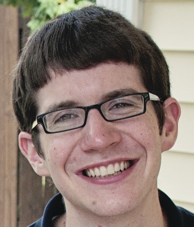 Greg Gandenberger
Philosopher of Science
University of Pittsburgh
gandenberger.org 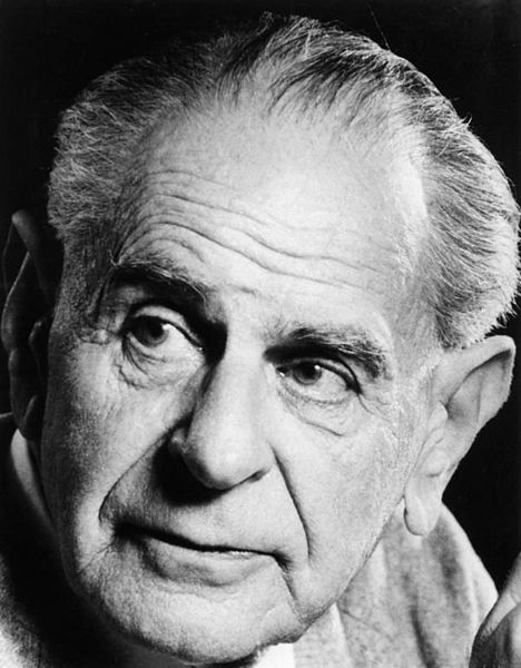
Genuine philosophical problems are always rooted in urgent problems outside philosophy,
and they die if these roots decay
Karl Popper (1963, 72)
My concern in this post is how we philosophers can use our skills to do work that matters to people both inside and outside of philosophy.
Philosophers are highly skilled at conceptual analysis, in which one takes an interesting but unclear concept and attempts to state precisely when it applies and when it doesn’t.
What is the point of this activity? In many cases, this question has no satisfactory answer. Conceptual analysis becomes an end in itself, and philosophical debates become fruitless arguments about words. The pleasure we philosophers take in such arguments hardly warrants scarce government and university resources. It does provide good training in critical thinking, but so do many other activities that are also immediately useful, such as doing science and programming computers.
Conceptual analysis does not have to be pointless. It is often prompted by a real-world problem. In Plato’s Euthyphro, for instance, the character Euthyphro thought that piety required him to prosecute his father for murder. His family thought on the contrary that for a son to prosecute his own father was the height of impiety. In this situation, the question “what is piety?” took on great urgency. It also had great urgency for Socrates, who was awaiting trial for corrupting the youth of Athens.
In general, conceptual analysis often begins as a response to some question about how we ought to regulate our beliefs or actions. It can be a fruitful activity as long as the questions that prompted it are kept in view. It tends to degenerate into merely verbal disputes when it becomes an end in itself.
The kind of goal-oriented view of conceptual analysis I aim to articulate and promote is not teleosemantics: it is a view about how philosophy should be done rather than a theory of meaning. It is consistent with Carnap’s notion of explication (one of the desiderata of which is fruitfulness) (Carnap 1963, 5), but in practice Carnapian explication seems to devolve into idle word games just as easily as conceptual analysis. Our overriding goal should not be fidelity to intuitions, precision, or systematicity, but usefulness.
How I Became Suspicious of Conceptual Analysis
When I began working on proofs of the Likelihood Principle, I assumed that following my intuitions about the concept of “evidential equivalence” would lead to insights about how science should be done. Birnbaum’s proof showed me that my intuitions entail the Likelihood Principle, which frequentist methods violate. Voila! Voila! Scientists shouldn’t use frequentist methods. All that remained to be done was to fortify Birnbaum’s proof, as I do in “A New Proof of the Likelihood Principle” by defending it against objections and buttressing it with an alternative proof. [Editor: For a number of related materials on this blog see Mayo’s JSM presentation, and note [i].]
After working on this topic for some time, I realized that I was making simplistic assumptions about the relationship between conceptual intuitions and methodological norms. At most, a proof of the Likelihood Principle can show you that frequentist methods run contrary to your intuitions about evidential equivalence. Even if those intuitions are true, it does not follow immediately that scientists should not use frequentist methods. The ultimate aim of science, presumably, is not to respect evidential equivalence but (roughly) to learn about the world and make it better. The demand that scientists use methods that respect evidential equivalence is warranted only insofar as it is conducive to achieving those ends. Birnbaum’s proof says nothing about that issue.
- In general, a conceptual analysis–even of a normatively freighted term like “evidence”–is never enough by itself to justify a normative claim. The questions that ultimately matter are not about “what we mean” when we use particular words and phrases, but rather about what our aims are and how we can best achieve them.
How to Do Conceptual Analysis Teleologically
This is not to say that my work on the Likelihood Principle or conceptual analysis in general is without value. But it is nothing more than a kind of careful lexicography. This kind of work is potentially useful for clarifying normative claims with the aim of assessing and possibly implementing them. To do work that matters, philosophers engaged in conceptual analysis need to take enough interest in the assessment and implementation stages to do their conceptual analysis with the relevant normative claims in mind.
So what does this kind of teleological (goal-oriented) conceptual analysis look like?
It can involve personally following through on the process of assessing and implementing the relevant norms. For example, philosophers at Carnegie Mellon University working on causation have not only provided a kind of analysis of the concept of causation but also developed algorithms for causal discovery, proved theorems about those algorithms, and applied those algorithms to contemporary scientific problems (see e.g. Spirtes et al. 2000).
I have great respect for this work. But doing conceptual analysis does not have to mean going so far outside the traditional bounds of philosophy. A perfect example is James Woodward’s related work on causal explanation, which he describes as follows (2003, 7-8, original emphasis):
My project…makes recommendations about what one ought to mean by various causal and explanatory claims, rather than just attempting to describe how we use those claims. It recognizes that causal and explanatory claims sometimes are confused, unclear, and ambiguous and suggests how those limitations might be addressed…. we introduce concepts…and characterize them in certain ways…because we want to do things with them…. Concepts can be well or badly designed for such purposes, and we can evaluate them accordingly.
Woodward keeps his eye on what the notion of causation is for, namely distinguishing between relationships that do and relationships that do not remain invariant under interventions. This distinction is enormously important because only relationships that remain invariant under interventions provide “handles” we can use to change the world.
Here are some lessons about teleological conceptual analysis that we can take from Woodward’s work. (I’m sure this list could be expanded.)
- Teleological conceptual analysis puts us in charge. In his wonderful presidential address at the 2012 meeting of the Philosophy of Science Association, Woodward ended a litany of metaphysical arguments against regarding mental events as causes by asking “Who’s in charge here?” There is no ideal form of Causation to which we must answer. We are free to decide to use “causation” and related words in the ways that best serve our interests.
- Teleological conceptual analysis can be revisionary. If ordinary usage is not optimal, we can change it.
- The product of a teleological conceptual analysis need not be unique. Some philosophers reject Woodward’s account because they regard causation as a process rather than as a relationship among variables. But why do we need to choose? There could just be two different notions of causation. Woodward’s account captures one notion that is very important in science and everyday life. If it captures all of the causal notions that are important, then so much the better. But this kind of comprehensiveness is not essential.
- Teleological conceptual analysis can be non-reductive. Woodward characterizes causal relations as (roughly) correlation relations that are invariant under certain kinds of interventions. But the notion of an intervention is itself causal. Woodward’s account is not circular because it characterizes what it means for a causal relationship to hold between two variables in terms of a different causal processes involving different sets of variables. But it is non-reductive in the sense that does not allow us to replace causal claims with equivalent non-causal claims (as, e.g., counterfactual, regularity, probabilistic, and process theories purport to do). This fact is a problem if one’s primary concern is to reduce one’s ultimate metaphysical commitments, but it is not necessarily a problem if one’s primary concern is to improve our ability to assess and use causal claims.
Conclusion
Philosophers rarely succeed in capturing all of our intuitions about an important informal concept. Even if they did succeed, they would have more work to do in justifying any norms that invoke that concept. Conceptual analysis can be a first step toward doing philosophy that matters, but it needs to be undertaken with the relevant normative claims in mind.
Question: What are your best examples of philosophy that matters? What can we learn from them?
Citations
- Birnbaum, Allan. “On the Foundations of Statistical Inference.” Journal of the American Statistical Association 57.298 (1962): 269-306.
- Carnap, Rudolf. Logical Foundations of Probability. U of Chicago Press, 1963.
- Gandenberger, Greg. “A New Proof of the Likelihood Principle.” The British Journal for the Philosophy of Science (forthcoming).
- Plato. Euthyphro. http://classics.mit.edu/Plato/euthyfro.html.
- Popper, Karl. Conjectures and Refutations. London: Routledge & Kegan Paul, 1963.
- Spirtes, Peter, Clark Glymour, and Richard Scheines. Causation, Prediction, and Search. Vol. 81. The MIT Press, 2000.
- Woodward, James. Making Things Happen: A Theory of Causal Explanation. Oxford University Press, 2003.
[i] Earlier posts are here and here. Some U-Phils are here, here, and here. For some amusing notes (e.g., Don’t Birnbaumize that experiment my friend, and Midnight with Birnbaum).
Some related papers:
- Mayo, D. G. (2012). “Statistical Science Meets Philosophy of Science Part 2: Shallow versus Deep Explorations”, Rationality, Markets, and Morals (RMM) 3, Special Topic: Statistical Science and Philosophy of Science, 71–107.
- Mayo, D. G. (2011) “Statistical Science and Philosophy of Science: Where Do/Should They Meet in 2011 (and beyond).” Rationality, Markets and Morals (RMM) 2, Special Topic: Statistical Science and Philosophy of Science, 79–102.
- Mayo, D. G. (2010). “An Error in the Argument from Conditionality and Sufficiency to the Likelihood Principle” in Error and Inference: Recent Exchanges on Experimental Reasoning, Reliability and the Objectivity and Rationality of Science (D Mayo and A. Spanos eds.), Cambridge: Cambridge University Press: 305-14.
- Cox D. R. and Mayo. D. G. (2010). “Objectivity and Conditionality in Frequentist Inference” in Error and Inference: Recent Exchanges on Experimental Reasoning, Reliability and the Objectivity and Rationality of Science (D Mayo and A. Spanos eds.), Cambridge: Cambridge University Press: 276-304.
A. Spanos: Egon Pearson’s Neglected Contributions to Statistics
 With permission from my colleague Aris Spanos, I reblog his (8/18/12): “Egon Pearson’s Neglected Contributions to Statistics“. It illuminates a different area of E.S.P’s work than my posts here and here.
Egon Pearson (11 August 1895 – 12 June 1980), is widely known today for his contribution in recasting of Fisher’s significance testing into the Neyman-Pearson (1933) theory of hypothesis testing. Occasionally, he is also credited with contributions in promoting statistical methods in industry and in the history of modern statistics; see Bartlett (1981). What is rarely mentioned is Egon’s early pioneering work on:
(i) specification: the need to state explicitly the inductive premises of one’s inferences,
(ii) robustness: evaluating the ‘sensitivity’ of inferential procedures to departures from the Normality assumption, as well as
(iii) Mis-Specification (M-S) testing: probing for potential departures from the Normality assumption.
Arguably, modern frequentist inference began with the development of various finite sample inference procedures, initially by William Gosset (1908) [of the Student’s t fame] and then Fisher (1915, 1921, 1922a-b). These inference procedures revolved around a particular statistical model, known today as the simple Normal model:
Xk ∽ NIID(μ,σ²), k=1,2,…,n,… (1)
where ‘NIID(μ,σ²)’ stands for ‘Normal, Independent and Identically Distributed with mean μ and variance σ²’. These procedures include the ‘optimal’ estimators of μ and σ², Xbar and s², and the pivotal quantities:
(a) τ(X) =[√n(Xbar- μ)/s] ∽ St(n-1), (2)
(b) v(X) =[(n-1)s²/σ²] ∽ χ²(n-1), (3)
where St(n-1) and χ²(n-1) denote the Student’s t and chi-square distributions with (n-1) degrees of freedom.
The question of ‘how these inferential results might be affected when the Normality assumption is false’ was originally raised by Gosset in a letter to Fisher in 1923:
“What I should like you to do is to find a solution for some other population than a normal one.” (Lehmann, 1999)
He went on to say that he tried the rectangular (uniform) distribution but made no progress, and he was seeking Fisher’s help in tackling this ‘robustness/sensitivity’ problem. In his reply that was unfortunately lost, Fisher must have derived the sampling distribution of τ(X), assuming some skewed distribution (possibly log-Normal). We know this from Gosset’s reply:
“I like the result for z [τ(X)] in the case of that horrible curve you are so fond of. I take it that in skew curves the distribution of z is skew in the opposite direction.” (Lehmann, 1999)
After this exchange Fisher was not particularly receptive to Gosset’s requests to address the problem of working out the implications of non-Normality for the Normal-based inference procedures; t, chi-square and F tests.
In contrast, Egon Pearson shared Gosset’s concerns about the robustness of Normal-based inference results (a)-(b) to non-Normality, and made an attempt to address the problem in a series of papers in the late 1920s and early 1930s. This line of research for Pearson began with a review of Fisher’s 2nd edition of the 1925 book, published in Nature, and dated June 8th, 1929. Pearson, after praising the book for its path breaking contributions, dared raise a mild criticism relating to (i)-(ii) above:
“There is one criticism, however, which must be made from the statistical point of view. A large number of tests are developed upon the assumption that the population sampled is of ‘normal’ form. That this is the case may be gathered from a very careful reading of the text, but the point is not sufficiently emphasised. It does not appear reasonable to lay stress on the ‘exactness’ of tests, when no means whatever are given of appreciating how rapidly they become inexact as the population samples diverge from normality.” (Pearson, 1929a)
Fisher reacted badly to this criticism and was preparing an acerbic reply to the ‘young pretender’ when Gosset jumped into the fray with his own letter in Nature, dated July 20th, in an obvious attempt to moderate the ensuing fight. Gosset succeeded in tempering Fisher’s reply, dated August 17th, forcing him to provide a less acerbic reply, but instead of addressing the ‘robustness/sensitivity’ issue, he focused primarily on Gosset’s call to address ‘the problem of what sort of modification of my tables for the analysis of variance would be required to adapt that process to non-normal distributions’. He described that as a hopeless task. This is an example of Fisher’s genious when cornered by an insightful argument. He sidestepped the issue of ‘robustness’ to departures from Normality, by broadening it – alluding to other possible departures from the ID assumption – and rendering it a hopeless task, by focusing on the call to ‘modify’ the statistical tables for all possible non-Normal distributions; there is an infinity of potential modifications!
Egon Pearson recognized the importance of stating explicitly the inductive premises upon which the inference results are based, and pressed ahead with exploring the robustness issue using several non-Normal distributions within the Pearson family. His probing was based primarily on simulation, relying on tables of pseudo-random numbers; see Pearson and Adyanthaya (1928, 1929), Pearson (1929b, 1931). His broad conclusions were that the t-test:
τ0(X)=|[√n(X-bar- μ0)/s]|, C1:={x: τ0(x) > cα}, (4)
for testing the hypotheses:
H0: μ = μ0 vs. H1: μ ≠ μ0, (5)
is relatively robust to certain departures from Normality, especially when the underlying distribution is symmetric, but the ANOVA test is rather sensitive to such departures! He continued this line of research into his 80s; see Pearson and Please (1975).
Perhaps more importantly, Pearson (1930) proposed a test for the Normality assumption based on the skewness and kurtosis coefficients: a Mis-Specification (M-S) test. Ironically, Fisher (1929) provided the sampling distributions of the sample skewness and kurtosis statistics upon which Pearson’s test was based. Pearson continued sharpening his original M-S test for Normality, and his efforts culminated with the D’Agostino and Pearson (1973) test that is widely used today; see also Pearson et al. (1977). The crucial importance of testing Normality stems from the fact that it renders the ‘robustness/sensitivity’ problem manageable. The test results can be used to narrow down the possible departures one needs to worry about. They can also be used to suggest ways to respecify the original model.
After Pearson’s early publications on the ‘robustness/sensitivity’ problem Gosset realized that simulation alone was not effective enough to address the question of robustness, and called upon Fisher, who initially rejected Gosset’s call by saying ‘it was none of his business’, to derive analytically the implications of non-Normality using different distributions:
“How much does it [non-Normality] matter? And in fact that is your business: none of the rest of us have the slightest chance of solving the problem: we can play about with samples [i.e. perform simulation studies], I am not belittling E. S. Pearson’s work, but it is up to you to get us a proper solution.” (Lehmann, 1999).
In this passage one can discern the high esteem with which Gosset held Fisher for his technical ability. Fisher’s reply was rather blunt:
“I do not think what you are doing with nonnormal distributions is at all my business, and I doubt if it is the right approach. … Where I differ from you, I suppose, is in regarding normality as only a part of the difficulty of getting data; viewed in this collection of difficulties I think you will see that it is one of the least important.”
It’s clear from this that Fisher understood the problem of how to handle departures from Normality more broadly than his contemporaries. His answer alludes to two issues that were not well understood at the time:
(a) departures from the other two probabilistic assumptions (IID) have much more serious consequences for Normal-based inference than Normality, and
(b) deriving the consequences of particular forms of non-Normality on the reliability of Normal-based inference, and proclaiming a procedure enjoys a certain level of ‘generic’ robustness, does not provide a complete answer to the problem of dealing with departures from the inductive premises.
In relation to (a) it is important to note that the role of ‘randomness’, as it relates to the IID assumptions, was not well understood until the 1940s, when the notion of non-IID was framed in terms of explicit forms of heterogeneity and dependence pertaining to stochastic processes. Hence, the problem of assessing departures from IID was largely ignored at the time, focusing almost exclusively on departures from Normality. Indeed, the early literature on nonparametric inference retained the IID assumptions and focused on inference procedures that replace the Normality assumption with indirect distributional assumptions pertaining to the ‘true’ but unknown f(x), like the existence of certain moments, its symmetry, smoothness, continuity and/or differentiability, unimodality, etc. ; see Lehmann (1975). It is interesting to note that Egon Pearson did not consider the question of testing the IID assumptions until his 1963 paper.
In relation to (b), when one poses the question ‘how robust to non-Normality is the reliability of inference based on a t-test?’ one ignores the fact that the t-test might no longer be the ‘optimal’ test under a non-Normal distribution. This is because the sampling distribution of the test statistic and the associated type I and II error probabilities depend crucially on the validity of the statistical model assumptions. When any of these assumptions are invalid, the relevant error probabilities are no longer the ones derived under the original model assumptions, and the optimality of the original test is called into question. For instance, assuming that the ‘true’ distribution is uniform (Gosset’s rectangular):
Xk ∽ U(a-μ,a+μ), k=1,2,…,n,… (6)
where f(x;a,μ)=(1/(2μ)), (a-μ) ≤ x ≤ (a+μ), μ > 0,
how does one assess the robustness of the t-test? One might invoke its generic robustness to symmetric non-Normal distributions and proceed as if the t-test is ‘fine’ for testing the hypotheses (5). A more well-grounded answer will be to assess the discrepancy between the nominal (assumed) error probabilities of the t-test based on (1) and the actual ones based on (6). If the latter approximate the former ‘closely enough’, one can justify the generic robustness. These answers, however, raise the broader question of what are the relevant error probabilities? After all, the optimal test for the hypotheses (5) in the context of (6), is no longer the t-test, but the test defined by:
w(X)=|{(n-1)([X[1] +X[n]]-μ0)}/{[X[1]-X[n]]}|∽F(2,2(n-1)), (7)
with a rejection region C1:={x: w(x) > cα}, where (X[1], X[n]) denote the smallest and the largest element in the ordered sample (X[1], X[2],…, X[n]), and F(2,2(n-1)) the F distribution with 2 and 2(n-1) degrees of freedom; see Neyman and Pearson (1928). One can argue that the relevant comparison error probabilities are no longer the ones associated with the t-test ‘corrected’ to account for the assumed departure, but those associated with the test in (7). For instance, let the t-test have nominal and actual significance level, .05 and .045, and power at μ1=μ0+1, of .4 and .37, respectively. The conventional wisdom will call the t-test robust, but is it reliable (effective) when compared with the test in (7) whose significance level and power (at μ1) are say, .03 and .9, respectively?
A strong case can be made that a more complete approach to the statistical misspecification problem is:
(i) to probe thoroughly for any departures from all the model assumptions using trenchant M-S tests, and if any departures are detected,
(ii) proceed to respecify the statistical model by choosing a more appropriate model with a view to account for the statistical information that the original model did not.
Admittedly, this is a more demanding way to deal with departures from the underlying assumptions, but it addresses the concerns of Gosset, Egon Pearson, Neyman and Fisher much more effectively than the invocation of vague robustness claims; see Spanos (2010).
References
Bartlett, M. S. (1981) “Egon Sharpe Pearson, 11 August 1895-12 June 1980,” Biographical Memoirs of Fellows of the Royal Society, 27: 425-443.
D’Agostino, R. and E. S. Pearson (1973) “Tests for Departure from Normality. Empirical Results for the Distributions of b₂ and √(b₁),” Biometrika, 60: 613-622.
Fisher, R. A. (1915) “Frequency distribution of the values of the correlation coefficient in samples from an indefinitely large population,” Biometrika, 10: 507-521.
Fisher, R. A. (1921) “On the “probable error” of a coefficient of correlation deduced from a small sample,” Metron, 1: 3-32.
Fisher, R. A. (1922a) “On the mathematical foundations of theoretical statistics,” Philosophical Transactions of the Royal Society A, 222, 309-368.
Fisher, R. A. (1922b) “The goodness of fit of regression formulae, and the distribution of regression coefficients,” Journal of the Royal Statistical Society, 85: 597-612.
Fisher, R. A. (1925) Statistical Methods for Research Workers, Oliver and Boyd, Edinburgh.
Fisher, R. A. (1929), “Moments and Product Moments of Sampling Distributions,” Proceedings of the London Mathematical Society, Series 2, 30: 199-238.
Neyman, J. and E. S. Pearson (1928) “On the use and interpretation of certain test criteria for purposes of statistical inference: Part I,” Biometrika, 20A: 175-240.
Neyman, J. and E. S. Pearson (1933) “On the problem of the most efficient tests of statistical hypotheses”, Philosophical Transanctions of the Royal Society, A, 231: 289-337.
Lehmann, E. L. (1975) Nonparametrics: statistical methods based on ranks, Holden-Day, San Francisco.
Lehmann, E. L. (1999) “‘Student’ and Small-Sample Theory,” Statistical Science, 14: 418-426.
Pearson, E. S. (1929a) “Review of ‘Statistical Methods for Research Workers,’ 1928, by Dr. R. A. Fisher”, Nature, June 8th, pp. 866-7.
Pearson, E. S. (1929b) “Some notes on sampling tests with two variables,” Biometrika, 21: 337-60.
Pearson, E. S. (1930) “A further development of tests for normality,” Biometrika, 22: 239-49.
Pearson, E. S. (1931) “The analysis of variance in cases of non-normal variation,” Biometrika, 23: 114-33.
Pearson, E. S. (1963) “Comparison of tests for randomness of points on a line,” Biometrika, 50: 315-25.
Pearson, E. S. and N. K. Adyanthaya (1928) “The distribution of frequency constants in small samples from symmetrical populations,” Biometrika, 20: 356-60.
Pearson, E. S. and N. K. Adyanthaya (1929) “The distribution of frequency constants in small samples from non-normal symmetrical and skew populations,” Biometrika, 21: 259-86.
Pearson, E. S. and N. W. Please (1975) “Relations between the shape of the population distribution and the robustness of four simple test statistics,” Biometrika, 62: 223-241.
Pearson, E. S., R. B. D’Agostino and K. O. Bowman (1977) “Tests for departure from normality: comparisons of powers,” Biometrika, 64: 231-246.
Spanos, A. (2010) “Akaike-type Criteria and the Reliability of Inference: Model Selection vs. Statistical Model Specification,” Journal of Econometrics, 158: 204-220.
Student (1908), “The Probable Error of the Mean,” Biometrika, 6: 1-25.
Blogging E.S. Pearson’s Statistical Philosophy
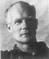
E.S. Pearson
For a bit more on the statistical philosophy of Egon Sharpe (E.S.) Pearson (11 Aug, 1895-12 June, 1980), I reblog a post from last year. It gets to the question I now call: performance or probativeness?
Are frequentist methods mainly useful to supply procedures which will not err too frequently in some long run? (performance) Or is it the other way round: that the control of long run error properties are of crucial importance for probing causes of the data at hand? (probativeness). I say no to the former and yes to the latter. This I think was also the view of Egon Pearson.
(i) Cases of Type A and Type B
“How far then, can one go in giving precision to a philosophy of statistical inference?” (Pearson 1947, 172)
Pearson considers the rationale that might be given to N-P tests in two types of cases, A and B:
“(A) At one extreme we have the case where repeated decisions must be made on results obtained from some routine procedure…
(B) At the other is the situation where statistical tools are applied to an isolated investigation of considerable importance…?” (ibid., 170)
In cases of type A, long-run results are clearly of interest, while in cases of type B, repetition is impossible and may be irrelevant:
“In other and, no doubt, more numerous cases there is no repetition of the same type of trial or experiment, but all the same we can and many of us do use the same test rules to guide our decision, following the analysis of an isolated set of numerical data. Why do we do this? What are the springs of decision? Is it because the formulation of the case in terms of hypothetical repetition helps to that clarity of view needed for sound judgment?
Or is it because we are content that the application of a rule, now in this investigation, now in that, should result in a long-run frequency of errors in judgment which we control at a low figure?” (Ibid., 173)
Although Pearson leaves this tantalizing question unanswered, claiming, “On this I should not care to dogmatize”, in studying how Pearson treats cases of type B, it is evident that in his view, “the formulation of the case in terms of hypothetical repetition helps to that clarity of view needed for sound judgment” in learning about the particular case at hand.
“Whereas when tackling problem A it is easy to convince the practical man of the value of a probability construct related to frequency of occurrence, in problem B the argument that ‘if we were to repeatedly do so and so, such and such result would follow in the long run’ is at once met by the commonsense answer that we never should carry out a precisely similar trial again.
Nevertheless, it is clear that the scientist with a knowledge of statistical method behind him can make his contribution to a round-table discussion…” (Ibid., 171).
Pearson gives the following example of a case of type B (from his wartime work), where he claims no repetition is intended:
“Example of type B. Two types of heavy armour-piercing naval shell of the same caliber are under consideration; they may be of different design or made by different firms…. Twelve shells of one kind and eight of the other have been fired; two of the former and five of the latter failed to perforate the plate….”(Pearson 1947, 171)
“Starting from the basis that, individual shells will never be identical in armour-piercing qualities, however good the control of production, he has to consider how much of the difference between (i) two failures out of twelve and (ii) five failures out of eight is likely to be due to this inevitable variability. ..”(Ibid.,)
As a noteworthy aside, Pearson shows that treating the observed difference (between the two proportions) in one way yields an observed significance level of 0.052; treating it differently (along Barnard’s lines), he gets 0.025 as the (upper) significance level. But in scientific cases, Pearson insists, the difference in error probabilities makes no real difference to substantive judgments in interpreting the results. Only in an unthinking, automatic, routine use of tests would it matter:
“Were the action taken to be decided automatically by the side of the 5% level on which the observation point fell, it is clear that the method of analysis used would here be of vital importance. But no responsible statistician, faced with an investigation of this character, would follow an automatic probability rule.” (ibid., 192)
The two analyses correspond to the tests effectively asking different questions, and if we recognize this, says Pearson, different meanings may be appropriately attached.
(ii) Three Steps in the Original construction of Tests
After setting up the test (or null) hypothesis, and the alternative hypotheses against which “we wish the test to have maximum discriminating power” (Pearson 1947, 173), Pearson defines three steps in specifying tests:
“Step 1. We must specify the experimental probability set, the set of results which could follow on repeated application of the random process used in the collection of the data…
Step 2. We then divide this set [of possible results] by a system of ordered boundaries…such that as we pass across one boundary and proceed to the next, we come to a class of results which makes us more and more inclined on the Information available, to reject the hypothesis tested in favour of alternatives which differ from it by increasing amounts” (Pearson 1966a, 173).
“Step 3. We then, if possible[i], associate with each contour level the chance that, if [the null] is true, a result will occur in random sampling lying beyond that level” (ibid.).
Pearson warns that:
“Although the mathematical procedure may put Step 3 before 2, we cannot put this into operation before we have decided, under Step 2, on the guiding principle to be used in choosing the contour system. That is why I have numbered the steps in this order.” (Ibid. 173).
Strict behavioristic formulations jump from step 1 to step 3, after which one may calculate how the test has in effect accomplished step 2. However, the resulting test, while having adequate error probabilities, may have an inadequate distance measure and may even be irrelevant to the hypothesis of interest. This is one reason critics can construct howlers that appear to be licensed by N-P methods, and which make their way from time to time into this blog.
So step 3 remains crucial, even for cases of type [B]. There are two reasons: pre-data planning—that’s familiar enough—but secondly, for post-data scrutiny. Post data, step 3 enables determining the capability of the test to have detected various discrepancies, departures, and errors, on which a critical scrutiny of the inferences are based. More specifically, the error probabilities are used to determine how well/poorly corroborated, or how severely tested, various claims are, post-data.
If we can readily bring about statistically significantly higher rates of success with the first type of armour-piercing naval shell than with the second (in the above example), we have evidence the first is superior. Or, as Pearson modestly puts it: the results “raise considerable doubts as to whether the performance of the [second] type of shell was as good as that of the [first]….” (Ibid., 192)[ii]
Still, while error rates of procedures may be used to determine how severely claims have/have not passed they do not automatically do so—hence, again, opening the door to potential howlers that neither Egon nor Jerzy for that matter would have countenanced.
(iii) Neyman Was the More Behavioristic of the Two
Pearson was (rightly) considered to have rejected the more behaviorist leanings of Neyman.
Here’s a snippet from an unpublished letter he wrote to Birnbaum (1974) about the idea that the N-P theory admits of two interpretations: behavioral and evidential:
“I think you will pick up here and there in my own papers signs of evidentiality, and you can say now that we or I should have stated clearly the difference between the behavioral and evidential interpretations. Certainly we have suffered since in the way the people have concentrated (to an absurd extent often) on behavioral interpretations”.
In Pearson’s (1955) response to Fisher (blogged last time):
“To dispel the picture of the Russian technological bogey, I might recall how certain early ideas came into my head as I sat on a gate overlooking an experimental blackcurrant plot….!” (Pearson 1955, 204)
“To the best of my ability I was searching for a way of expressing in mathematical terms what appeared to me to be the requirements of the scientist in applying statistical tests to his data. After contact was made with Neyman in 1926, the development of a joint mathematical theory proceeded much more surely; it was not till after the main lines of this theory had taken shape with its necessary formalization in terms of critical regions, the class of admissible hypotheses, the two sources of error, the power function, etc., that the fact that there was a remarkable parallelism of ideas in the field of acceptance sampling became apparent. Abraham Wald’s contributions to decision theory of ten to fifteen years later were perhaps strongly influenced by acceptance sampling problems, but that is another story.“ (ibid., 204-5).
“It may be readily agreed that in the first Neyman and Pearson paper of 1928, more space might have been given to discussing how the scientific worker’s attitude of mind could be related to the formal structure of the mathematical probability theory….Nevertheless it should be clear from the first paragraph of this paper that we were not speaking of the final acceptance or rejection of a scientific hypothesis on the basis of statistical analysis…. Indeed, from the start we shared Professor Fisher’s view that in scientific enquiry, a statistical test is ‘a means of learning”… (Ibid., 206)
“Professor Fisher’s final criticism concerns the use of the term ‘inductive behavior’; this is Professor Neyman’s field rather than mine.” (Ibid., 207)
__________________________
Aside: It is interesting, given these non-behavioristic leanings that Pearson had earlier worked in acceptance sampling and quality control (from which he claimed to have obtained the term “power”). From the Cox-Mayo “conversation” (2011, 110):
COX: It is relevant that Egon Pearson had a very strong interest in industrial design and quality control.
MAYO: Yes, that’s surprising, given his evidential leanings and his apparent dis-taste for Neyman’s behavioristic stance. I only discovered that around 10 years ago; he wrote a small book.[iii]
COX: He also wrote a very big book, but all copies were burned in one of the first air raids on London.
Some might find it surprising to learn that it is from this early acceptance sampling work that Pearson obtained the notion of “power”, but I don’t have the quote handy where he said this……
References:
Cox, D. and Mayo, D. G. (2011), “Statistical Scientist Meets a Philosopher of Science: A Conversation,” Rationality, Markets and Morals: Studies at the Intersection of Philosophy and Economics, 2: 103-114.
Pearson, E. S. (1935), The Application of Statistical Methods to Industrial Standardization and Quality Control, London: British Standards Institution.
Pearson, E. S. (1947), “The choice of Statistical Tests illustrated on the Interpretation of Data Classed in a 2×2 Table,” Biometrika 34(1/2): 139-167.
Pearson, E. S. (1955), “Statistical Concepts and Their Relationship to Reality” Journal of the Royal Statistical Society, Series B, (Methodological), 17(2): 204-207.
Neyman, J. and Pearson, E. S. (1928), “On the Use and Interpretation of Certain Test Criteria for Purposes of Statistical Inference, Part I.” Biometrika 20(A): 175-240.
E.S. Pearson: “Ideas came into my head as I sat on a gate overlooking an experimental blackcurrant plot”
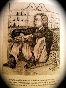
E.S.Pearson on a Gate, Mayo sketch
Today is Egon Pearson’s birthday (11 Aug., 1895-12 June, 1980); and here you see my scruffy sketch of him, at the start of my book, “Error and the Growth of Experimental Knowledge” (EGEK 1996). As Erich Lehmann put it in his EGEK review, Pearson is “the hero of Mayo’s story” because I found in his work, if only in brief discussions, hints, and examples, the key elements for an “inferential” or “evidential” interpretation of Neyman-Pearson theory of statistics. “Pearson and Pearson” statistics (both Egon, not Karl) would have looked very different from Neyman and Pearson statistics, I suspect. One of the few sources of E.S. Pearson’s statistical philosophy is his (1955) “Statistical Concepts in Their Relation to Reality”. It begins like this:
Controversies in the field of mathematical statistics seem largely to have arisen because statisticians have been unable to agree upon how theory is to provide, in terms of probability statements, the numerical measures most helpful to those who have to draw conclusions from observational data. We are concerned here with the ways in which mathematical theory may be put, as it were, into gear with the common processes of rational thought, and there seems no reason to suppose that there is one best way in which this can be done. If, therefore, Sir Ronald Fisher recapitulates and enlarges on his views upon statistical methods and scientific induction we can all only be grateful, but when he takes this opportunity to criticize the work of others through misapprehension of their views as he has done in his recent contribution to this Journal (Fisher 1955 “Scientific Methods and Scientific Induction” ), it is impossible to leave him altogether unanswered.
In the first place it seems unfortunate that much of Fisher’s criticism of Neyman and Pearson’s approach to the testing of statistical hypotheses should be built upon a “penetrating observation” ascribed to Professor G.A. Barnard, the assumption involved in which happens to be historically incorrect. There was no question of a difference in point of view having “originated” when Neyman “reinterpreted” Fisher’s early work on tests of significance “in terms of that technological and commercial apparatus which is known as an acceptance procedure”. There was no sudden descent upon British soil of Russian ideas regarding the function of science in relation to technology and to five-year plans. It was really much simpler–or worse. The original heresy, as we shall see, was a Pearson one!…
Indeed, to dispel the picture of the Russian technological bogey, I might recall how certain early ideas came into my head as I sat on a gate overlooking an experimental blackcurrant plot…!
To continue reading, “Statistical Concepts in Their Relation to Reality” click HERE.
See also Aris Spanos: “Egon Pearson’s Neglected Contributions to Statistics“.
Happy Birthday E.S. Pearson!
11th bullet, multiple choice question, and last thoughts on the JSM
 I. Apparently I left out the last bullet in my scribbled notes from Silver’s talk. There was an 11th. Someone sent it to me from a blog: revolution analytics:
11. Like scientists, journalists ought to be more concerned with the truth rather than just appearances. He suggested that maybe they should abandon the legal paradigm of seeking an adversarial approach and behave more like scientists looking for the truth.
OK. But, given some of the issues swirling around the last few posts, I think it’s worth noting that scientists are not disinterested agents looking for the truth—it’s only thanks to its (adversarial!) methods that they advance upon truth. Question: What’s the secret of scientific progress (in those areas that advance learning)? Answer: Even if each individual scientist were to strive mightily to ensure that his/her theory wins out, the stringent methods of the enterprise force that theory to show its mettle or die (or at best remain in limbo). You might say, “But there are plenty of stubborn hard cores in science”. Sure, and they fail to advance. In those sciences that lack sufficiently stringent controls, the rate of uncorrected spin is as bad as Silver suggests it is in journalism. Think of social psychologist Diederik Stapel setting out to show what is already presumed to be believable. (See here and here and search this blog.).
There’s a strange irony when the same people who proclaim, “We must confront those all too human flaws and foibles that obstruct the aims of truth and correctness”, turn out to be enablers, by championing methods that enable flaws and foibles to seep through. It may be a slip of logic. Here’s a multiple choice question:
Multiple choice: Circle all phrases that correctly complete the “conclusion“:
Let’s say that factor F is known to obstruct the correctness/validity of solutions to problems, or that factor F is known to adversely impinge on inferences.
(Examples of such factors include: biases, limited information, incentives—of various sorts).
Factor F is known to adversely influence inferences.
Conclusion: Therefore any adequate systematic account of inference should _______
(a) allow F to influence inferences.
(b) provide a formal niche by which F can influence inferences.
(c) take precautions to block (or at least be aware of) the ability of F to adversely influence inferences.
(d) none of the above.
(For an example, see discussion of #7 in previous post.)
II. I may be overlooking sessions (inform me if you know of any), but I would have expected more on the statistics in the Higgs boson discoveries at the JSM 2013. Especially given the desire to emphasize the widespread contributions of statistics to the latest sexy science[i]. (At one point, I was asked about being part of a session on the five sigma effect in the Higgs boson discovery–not that I’m any kind of expert– by David Banks, because of my related blog posts (e.g., here), but people were already in other sessions. But I’m thinking about something splashy by statisticians in particle physics.) Did I miss? [ii]
III. I think it’s easy to see why lots of people showed up to hear Nate Silver: It’s fun to see someone “in the news”, be it from politics, finance, high tech, acting, TV, or, even academics–I, for one, was curious. I’m sure as many would have come out to hear Esther Duflo, Cheryl Sandberg, Fabiola Gionatti, or even Huma Abedin–to list some that happen to come to mind– or any number of others who have achieved recent recognition (and whose work intersects in some way with statistics). It’s interesting that I don’t see pop philosophers invited to give key addresses in yearly philosophy meetings; maybe because philosophers eschew popularity. I may be unaware of some; I don’t attend so many meetings.
IV. Other thoughts: I’ve only been to a handful of “official” statistics meetings. Obviously the # of simultaneous sessions makes the JSM a kind of factory experience, but that’s to be expected. But do people really need to purchase those JSM backpacks? I don’t know how much of the $400 registration fee goes to that, but it seems wasteful…. I saw people tossing theirs out, which I didn’t have the heart to do. Perhaps I’m just showing my outsider status.
V. Montreal: I intended to practice my French, but kept bursting into English too soon. Everyone I met (who lives there) complained about the new money and doing away with pennies in the near future. I wonder if we’re next.
[i]On Silver’s remark (in response to a “tweeted” question) that “data science” is a “sexed-up” term for statistics, I don’t know. I can see reflecting deeply over the foundations of statistical inference, but over the foundations of data analytics?
[ii] You don’t suppose the controversy about particle physics being “bad science” had anything to do with downplaying the Higgs statistics?
What did Nate Silver just say? Blogging the JSM
 Nate Silver gave his ASA Presidential talk to a packed audience (with questions tweeted[i]). Here are some quick thoughts—based on scribbled notes (from last night). Silver gave a list of 10 points that went something like this (turns out there were 11):
1. statistics are not just numbers
2. context is needed to interpret data
3. correlation is not causation
4. averages are the most useful tool
5. human intuitions about numbers tend to be flawed and biased
6. people misunderstand probability
7. we should be explicit about our biases and (in this sense) should be Bayesian?
8. complexity is not the same as not understanding
9. being in the in crowd gets in the way of objectivity
10. making predictions improves accountability
Just to comment on #7, I don’t know if this is a brand new philosophy of Bayesianism, but his position went like this: Journalists and others are incredibly biased, they view data through their prior conceptions, wishes, goals, and interests, and you cannot expect them to be self-critical enough to be aware of, let alone be willing to expose, their propensity toward spin, prejudice, etc. Silver said the reason he favors the Bayesian philosophy (yes he used the words “philosophy” and “epistemology”) is that people should be explicit about disclosing their biases. I have three queries: (1) If we concur that people are so inclined to see the world through their tunnel vision, what evidence is there that they are able/willing to be explicit about their biases? (2) If priors are to be understood as the way to be explicit about one’s biases, shouldn’t they be kept separate from the data rather than combined with them? (3) I don’t think this is how Bayesians view Bayesianism or priors—is it? Subjective Bayesians, I thought, view priors as representing prior or background information about the statistical question of interest; but Silver sees them as admissions of prejudice, bias or what have you. As a confession of bias, I’d be all for it—though I think people may be better at exposing other’s biases than their own. Only thing: I’d need an entirely distinct account of warranted inference from data.
This does possibly explain some inexplicable remarks in Silver’s book to the effect that R.A. Fisher denied, excluded, or overlooked human biases since he disapproved of adding subjective prior beliefs to data in scientific contexts. Is Silver just about to recognize/appreciate the genius of Fisher (and others) in developing techniques consciously designed to find things out despite knowledge gaps, variability, and human biases? Or not?
Share your comments and/or links to other blogs discussing his talk (which will surely be posted if it isn’t already). Fill in gaps if you were there—I was far away… (See also my previous post blogging the JSM). 
[i] What was the point of this, aside from permitting questions to be cherry picked? (It would have been fun to see ALL the queries tweeted.) The ones I heard were limited to: how can we make statistics more attractive, who is your favorite journalist, favorite baseball player, and so on. But I may have missed some, I left before the end.
For a follow-up post including an 11th bullet that I’d missed, see here. My first post on JSM13 (8/5/13) was here.
At the JSM: 2013 International Year of Statistics
 “2013 is the International Year of Statistics” the JSM (Joint Statistical Meetings) brochures ring out! What does it mean? Whatever it is, it’s exciting! Errorstatistics.com never took up this question, but it’s been on some of the blogs in my “Blog bagel”. So, Since I’m at the JSM here in Montreal, I may report on any clues. Please share your comments. I’m not a statistician, but a philosopher of science, and of inductive-statistical inference much more generally. So I have no dog in this fight, as they say. (Or do I? ) On the other hand, I have often rued “the decline of late in the lively and long-standing exchange between philosophers of science and statisticians” (see this post). [i] (We did have that one parody on “big data or pig data”.)
I know from Larry Wasserman (normaldeviate) that the “year of” label grows, at least in part, to help prevent Statistical Science being eclipsed by the fashionable “Big Data” crowd. In one blog he even spoke of “the end of statistics”. “Aren’t We Data Science?” Marie Davidian, president of the ASA, asks in a recent AmStatNews article.[ii] Davidian worries, correctly I’ve no doubt, that Big Dadaists may be collecting data with “little appreciation for the power of design principle. Statisticians could propel major advances through developments of ‘experimental design for the 21st century’!”. This recalls Stan Young’s recent post:
Until relatively recently, the microarray samples were not sent through assay equipment in random order. Clinical trial statisticians at GSK insisted that the samples go through assay in random order. Rather amazingly the data became less messy and p-values became more orderly. The story is given here: http://blog.goldenhelix.com/?p=322. Essentially all the microarray data pre-2010 is unreliable…..So often the problem is not with p-value technology, but with the design and conduct of the study.
So without statistical design principles, they may have wasted a decade!
Back to the JSM, I see they’ve even invited pollster Nate Silver to give the AMA presidential address. I thought he was more baseball stat expert/pundit/pollster than statistician, but some are calling him an “analytics rock star”. Never mind that there’s at least one extremely strange chapter (8) in his popular book (The Signal and the Noise). Here’s an excerpt from Wasserman’s review, which he titles: “Nate Silver is a Frequentist: Review of The signal and the noise”:
I have one complaint. Silver is a big fan of Bayesian inference, which is fine. Unfortunately, he falls into that category I referred to a few posts ago. He confuses ‘Bayesian inference’ with ‘using Bayes’ theorem.’ His description of frequentist inference is terrible. He seems to equate frequentist inference with Fisherian significance testing, most using Normal distributions. Either he learned statistics from a bad book or he hangs out with statisticians with a significant anti-frequentist bias. Have no doubt about it: Nate Silver is a frequentist.[iii] (Wasserman)
I didn’t discuss Silver’s book on this blog, but looking up a few comments I made on other blogs, (e.g.,on a Gelman blog reviewing Silver), I see I am a bit less generous than Wasserman: “Frequentists, Silver alleges, go around reporting hypotheses like toads predict earthquakes and other “manifestly ridiculous” findings that are licensed by significance testing and data dredged correlations. (Silver, 253). But it is the frequentist who prevents such spurious correlations…. “ (Mayo) So Silver’s criticisms of frequents are way off base. I was also slightly aghast at his Fisher ridicule and I poke fun at his “All-You-Need is Bayesian cheerleading. The simple use of Bayes Theorem solves all problems (he seems not to realize they too require statistical models)” I wrote. It’s hard to tell if he’s just reporting or chiming in with those who advocate that schools stop teaching frequentist methods. Some statistical self-inflicted wounds perhaps? The other chapters look interesting, though I didn’t get too much further…(The Bayesian examples are all ordinary frequentist updating, it appears.) If I can, I’ll go to Silver’s talk.
[i] In that post I wrote: “Philosophy of statistical science not only deals with the philosophical foundations of statistics but also questions about the nature of and justification for inductive-statistical learning more generally. So it is ironic that just as philosophy of science is striving to immerse itself in and be relevant to scientific practice, that statistical science and philosophy of science—so ahead of their time in combining the work of philosophers and practicing scientists—should see such dialogues become rather rare. (See special topic here.)” (Mayo)
[ii] Some of the turf battles I hear about appear to reflect less substance than style (i.e., people being galvanized to use the latest meme in funding opportunities). Even in philosophy, the dept. head asked us to try and work it in. In my view, rather than suggesting “Plato and Big Data”, they should be asking to highlight interconnections between statistical evidence, critical thinking, logic, ethics, philosophy of science, and epistemology. That would advance our courses.
[iii] For example, Wasserman says, in his review of Silver:
One of the most important tests of a forecast — I would argue that it is the single most important one — is called calibration. Out of all the times you said there was a 40 percent chance of rain, how often did rain actually occur? If over the long run, it really did rain about 40 percent of the time, that means your forecasts were well calibrated. (Wasserman)
Blogging (flogging?) the SLP: Response to Reply- Xi’an Robert

Breaking through “the breakthrough”
Christian Robert’s reply grows out of my last blogpost. On Xi’an’s Og :
A quick reply from my own Elba, in the Dolomiti: your arguments (about the sad consequences of the SLP) are not convincing wrt the derivation of SLP=WCP+SP. If I built a procedure that reports (E1,x*) whenever I observe (E1,x*) or (E2,y*), this obeys the sufficiency principle; doesn’t it? (Sorry to miss your talk!)
Mayo’s response to Xi’an on the “sad consequences of the SLP.”[i]
This is a useful reply (so to me it’s actually not ‘flogging’ the SLP[ii]), and, in fact, I think Xi’an will now see why my arguments are convincing! Let’s use Xi’an’s procedure to make a parametric inference about q. Getting the report x* from Xi’an’s procedure, we know it could have come from E1 or E2. In that case, the WCP forbids us from using either individual experiment to compute the inference implication. We use the sampling distribution of TB.
Birnbaum’s statistic TB is a technically sufficient statistic for Birnbaum’s experiment EB (the conditional distribution of Z given TB is independent of q). The question of whether this is the relevant or legitimate way to compute the inference when it is given that y* came from E2 is the big question. The WCP says it is not. Now you are free to use Xi’an’s procedure (free to Birnbaumize) but that does not yield the SLP. Nor did Birnbaum think it did. That’s why he goes on to say: “Never mind. Don’t use Xi’an’s procedure. Compute the inference using E2 just as the WCP tells you to. You know it came from E2 . Isn’t that what David Cox taught us in 1958?”
Fine. But still no SLP! Note it’s not that SP and WCP conflict, it’s WCP and Birnbaumization that conflict. The application of a principle will always be relative to the associated model used to frame the question.[iii]
These points are all spelled out clearly in my paper: [I can’t get double subscripts here. EB is the same as E-B][iv]
Given y*, the WCP says do not Birnbaumize. One is free to do so, but not to simultaneously claim to hold the WCP in relation to the given y*, on pain of logical contradiction. If one does choose to Birnbaumize, and to construct TB, admittedly, the known outcome y* yields the same value of TB as would x*. Using the sample space of EB yields: (B): InfrE-B[x*] = InfrE-B[y*]. This is based on the convex combination of the two experiments, and differs from both InfrE1[x*] and InfrE2[y*]. So again, any SLP violation remains. Granted, if only the value of TB is given, using InfrE-B may be appropriate. For then we are given only the disjunction: Either (E1, x*) or (E2, y*). In that case one is barred from using the implication from either individual Ei. A holder of WCP might put it this way: once (E,z) is given, whether E arose from a q-irrelevant mixture, or was fixed all along, should not matter to the inference; but whether a result was Birnbaumized or not should, and does, matter.
There is no logical contradiction in holding that if data are analyzed one way (using the convex combination in EB), a given answer results, and if analyzed another way (via WCP) one gets quite a different result. One may consistently apply both the EB and the WCP directives to the same result, in the same experimental model, only in cases where WCP makes no difference. To claim the WCP never makes a difference, however, would entail that there can be no SLP violations, which would make the argument circular. Another possibility, would be to hold, as Birnbaum ultimately did, that the SLP is “clearly plausible” (Birnbaum 1968, 301) only in “the severely restricted case of a parameter space of just two points” where these are predesignated (Birnbaum 1969, 128). But SLP violations remain.
Note: The final draft of my paper uses equations that do not transfer directly to this blog. Hence, these sections are from a draft of my paper.
[i] Although I didn’t call them “sad,” I think it would be too bad to accept the SLP’s consequences. Listen to Birnbaum:
The likelihood principle is incompatible with the main body of modern statistical theory and practice, notably the Neyman-Pearson theory of hypothesis testing and of confidence intervals, and incompatible in general even with such well-known concepts as standard error of an estimate and significance level. (Birnbaum 1968, 300)
That is why Savage called it “a breakthrough” result. In the end, however, Birnbaum could not give up on control of error probabilities. He held the SLP only for the trivial case of predesignated simple hypotheses. (Or, perhaps he spied the gap in his argument? I suspect, from his writings, that he realized his argument went through only for such cases that do not violate the SLP.)
[ii] Readers may feel differently.
[iii] Excerpt from a draft of my paper:
Model checking. An essential part of the statements of the principles SP, WCP, and SLP is that the validity of the model is granted as adequately representing the experimental conditions at hand (Birnbaum 1962, 491). Thus, accounts that adhere to the SLP are not thereby prevented from analyzing features of the data such as residuals, which are relevant to questions of checking the statistical model itself. There is some ambiguity on this point in Casella and R. Berger (2002):
Most model checking is, necessarily, based on statistics other than a sufficient statistic. For example, it is common practice to examine residuals from a model. . . Such a practice immediately violates the Sufficiency Principle, since the residuals are not based on sufficient statistics. (Of course such a practice directly violates the [strong] LP also.) (Casella and R. Berger 2002, 295-6)
They warn that before considering the SLP and WCP, “we must be comfortable with the model” (296). It seems to us more accurate to regard the principles as inapplicable, rather than violated, when the adequacy of the relevant model is lacking.
Birnbaum, A.1968. “Likelihood.” In International Encyclopedia of the Social Sciences, 9:299–301. New York: Macmillan and the Free Press.
———. 1969. “Concepts of Statistical Evidence.” In Philosophy, Science, and Method: Essays in Honor of Ernest Nagel, edited by S. Morgenbesser, P. Suppes, and M. G. White, 112–143. New York: St. Martin’s Press.
Casella, G., and R. L. Berger. 2002. Statistical Inference. 2nd ed. Belmont, CA: Duxbury Press.
Mayo 2013, (http://arxiv-web3.library.cornell.edu/pdf/1302.7021v2.pdf)
New Version: On the Birnbaum argument for the SLP: Slides for my JSM talk
 In my latest formulation of the controversial Birnbaum argument for the strong likelihood principle (SLP), I introduce a new symbol
(E,z)
A draft of my slides for the Joint Statistical Meetings JSM in Montreal next week are right after the abstract. Comments are very welcome.
Interested readers may search this blog for quite a lot of discussion of the SLP (e.g., here and here) including links to the central papers, “U-Phils” by others (e.g., here, here, and here), and amusing notes (e.g., Don’t Birnbaumize that experiment my friend, and Midnight with Birnbaum).
On the Birnbaum Argument for the Strong Likelihood Principle
Abstract
An essential component of inference based on familiar frequentist notions p-values, significance and confidence levels, is the relevant sampling distribution (hence the term sampling theory). This feature results in violations of a principle known as the strong likelihood principle (SLP), the focus of this paper. In particular, if outcomes x* and y* from experiments E1 and E2 (both with unknown parameter θ), have different probability models f1, f2, then even though f1(x*; θ) = cf2(y*; θ) for all θ, outcomes x* and y* may have different implications for an inference about θ. Although such violations stem from considering outcomes other than the one observed, we argue, this does not require us to consider experiments other than the one performed to produce the data. David Cox (1958) proposes the Weak Conditionality Principle (WCP) to justify restricting the space of relevant repetitions. The WCP says that once it is known which Ei produced the measurement, the assessment should be in terms of the properties of the particular Ei.
The surprising upshot of Allan Birnbaum’s (1962) argument is that the SLP appears to follow from applying the WCP in the case of mixtures, and so uncontroversial a principle as sufficiency (SP). But this would preclude the use of sampling distributions. The goal of this article is to provide a new clarification and critique of Birnbaum’s argument. Although his argument purports that [(WCP and SP) entails SLP], we show how data may violate the SLP while holding both the WCP and SP. Such cases directly refute [WCP entails SLP].
Comments, questions, errors are welcome.
Full paper can be found here: http://arxiv-web3.library.cornell.edu/abs/1302.7021
Background Knowledge: Not to Quantify, But To Avoid Being Misled By, Subjective Beliefs
 A low-powered statistical analysis of this blog—nearing its 2-year anniversary!—reveals that the topic to crop up most often—either front and center, or lurking in the bushes–is that of “background information”. The following was one of my early posts, back in Oct.30, 2011:
October 30, 2011 (London). Increasingly, I am discovering that one of the biggest sources of confusion about the foundations of statistics has to do with what it means or should mean to use “background knowledge” and “judgment” in making statistical and scientific inferences. David Cox and I address this in our “Conversation” in RMM (2011); it is one of the three or four topics in that special volume that I am keen to take up.
Insofar as humans conduct science and draw inferences, and insofar as learning about the world is not reducible to a priori deductions, it is obvious that “human judgments” are involved. True enough, but too trivial an observation to help us distinguish among the very different ways judgments should enter according to contrasting inferential accounts. When Bayesians claim that frequentists do not use or are barred from using background information, what they really mean is that frequentists do not use prior probabilities of hypotheses, at least when those hypotheses are regarded as correct or incorrect, if only approximately. So, for example, we would not assign relative frequencies to the truth of hypotheses such as (1) prion transmission is via protein folding without nucleic acid, or (2) the deflection of light is approximately 1.75” (as if, as Pierce puts it, “universes were as plenty as blackberries”). How odd it would be to try to model these hypotheses as themselves having distributions: to us, statistical hypotheses assign probabilities to outcomes or values of a random variable.
However, quite a lot of background information goes into designing, carrying out, and analyzing inquiries into hypotheses regarded as correct or incorrect. For a frequentist, that is where background knowledge enters. There is no reason to suppose that the background required in order sensibly to generate, interpret, and draw inferences about H should—or even can—enter through prior probabilities for H itself! Of course, presumably, Bayesians also require background information in order to determine that “data x” have been observed, to determine how to model and conduct the inquiry, and to check the adequacy of statistical models for the purposes of the inquiry. So the Bayesian prior only purports to add some other kind of judgment, about the degree of belief in H. It does not get away from the other background judgments that frequentists employ.
This relates to a second point that came up in our conversation when Cox asked, “Do we want to put in a lot of information external to the data, or as little as possible?” Continue reading
Guest Post: Larry Laudan. Why Presuming Innocence is Not a Bayesian Prior
 “Why presuming innocence has nothing to do with assigning low prior probabilities to the proposition that defendant didn’t commit the crime”
by Professor Larry Laudan
Philosopher of Science*
Several of the comments to the July 17 post about the presumption of innocence suppose that jurors are asked to believe, at the outset of a trial, that the defendant did not commit the crime and that they can legitimately convict him if and only if they are eventually persuaded that it is highly likely (pursuant to the prevailing standard of proof) that he did in fact commit it. Failing that, they must find him not guilty. Many contributors here are conjecturing how confident jurors should be at the outset about defendant’s material innocence.
That is a natural enough Bayesian way of formulating the issue but I think it drastically misstates what the presumption of innocence amounts to. In my view, the presumption is not (or at least should not be) an instruction about whether jurors believe defendant did or did not commit the crime. It is, rather, an instruction about their probative attitudes.
There are three reasons for thinking this:
a). asking a juror to begin a trial believing that defendant did not commit a crime requires a doxastic act that is probably outside the jurors’ control. It would involve asking jurors to strongly believe an empirical assertion for which they have no evidence whatsoever. It is wholly unclear that any of us has the ability to talk ourselves into resolutely believing x if we have no empirical grounds for asserting x. By contrast, asking juries to believe that they have seen as yet no proof of defendant’s guilt is an easy belief to acquiesce in since it is obviously true. Continue reading
Msc Kvetch: A question on the Martin-Zimmerman case we do not hear
 This is off topic, but a question I don’t hear people ask in regard to the Zimmerman case is: why didn’t any of the several people hearing screams intervene to stop the brawl? Never mind who was screaming, no one felt an obligation to intervene. Eye-witness John Good came out and said something like “stop” but then immediately ran back inside. Others could be heard saying, “don’t go out there”. I don’t say they should have joined the fight, but if a few people had gone outside and screamed or blew a whistle it probably would have been effective.
(I’ve been in such situations twice.)
Phil/Stat/Law: What Bayesian prior should a jury have? (Schachtman)
Nathan Schachtman, Esq., PC* emailed me the following interesting query a while ago:
When I was working through some of the Bayesian in the law issues with my class, I raised the problem of priors of 0 and 1 being off “out of bounds” for a Bayesian analyst. I didn’t realize then that the problem had a name: Cromwell’s Rule.
My point was then, and more so now, what is the appropriate prior the jury should have when it is sworn? When it hears opening statements? Just before the first piece of evidence is received?
Do we tell the jury that the defendant is presumed innocent, which means that it’s ok to entertain a very, very small prior probability of guilt, say no more than 1/N, where N is the total population of people? This seems wrong as a matter of legal theory. But if the prior = 0, then no amount of evidence can move the jury off its prior.

*Schachtman’s legal practice focuses on the defense of product liability suits, with an emphasis on the scientific and medico-legal issues. He teaches a course in statistics in the law at the Columbia Law School, NYC. He also has a legal blog here.
Stephen Senn: Indefinite irrelevance
 Stephen Senn
Head, Methodology and Statistics Group,
Competence Center for Methodology and Statistics (CCMS),
Luxembourg
At a workshop on randomisation I attended recently I was depressed to hear what I regard as hackneyed untruths treated as if they were important objections. One of these is that of indefinitely many confounders. The argument goes that although randomisation may make it probable that some confounders are reasonably balanced between the arms, since there are indefinitely many of these, the chance that at least some are badly confounded is so great as to make the procedure useless.
This argument is wrong for several related reasons. The first is to do with the fact that the total effect of these indefinitely many confounders is bounded. This means that the argument put forward is analogously false to one in which it were claimed that the infinite series ½, ¼,⅛ …. did not sum to a limit because there were infinitely many terms. The fact is that the outcome value one wishes to analyse poses a limit on the possible influence of the covariates. Suppose that we were able to measure a number of covariates on a set of patients prior to randomisation (in fact this is usually not possible but that does not matter here). Now construct principle components, C1, C2… .. based on these covariates. We suppose that each of these predict to a greater or lesser extent the outcome, Y (say). In a linear model we could put coefficients on these components, k1, k2… (say). However one is not free to postulate anything at all by way of values for these coefficients, since it has to be the case for any set of m such coefficients that  where V( ) indicates variance of. Thus variation in outcome bounds variation in prediction. This total variation in outcome has to be shared between the predictors and the more predictors you postulate there are, the less on average the influence per predictor.
The second error is to ignore the fact that statistical inference does not proceed on the basis of signal alone but also on noise. It is the ratio of these that is important. If there are indefinitely many predictors then there is no reason to suppose that their influence on the variation between treatment groups will be bigger than their variation within groups and both of these are used to make the inference. Continue reading
Professor of Philosophy Resigns over Sexual Misconduct (rejected post)
 My field (philosophy) is not known for the kinds of data frauds and retractions we’ve discussed on this blog, but scandals revolving around sexual harassment by male faculty are not rare, though I can’t think of another with a senior faculty resigning, at least not in recent times. This article is from
A Few Words on the McGinn Imbroglio from the philosophy smoker blog (June 4, 2013)
As I guess we [in philosophy] all know, Colin McGinn has chosen to resign from the University of Miami rather than allow the University to proceed with an investigation into allegations of sexual misconduct involving a research assistant. The article at the Chronicle of Higher Ed is here (paywalled); Sally Haslanger has posted a PDF of the whole thing here. Discussion at NewApps here, here, here, and here; discussion at Feminist Philosophers here; discussion at Leiter here and here.
Briefly, what seems to have happened is this: McGinn had a Research Assistant who was a female graduate student. Last spring, the RA started feeling uncomfortable with McGinn. Then, last April, McGinn allegedly started sending her sexually explicit email messages, including one in which, according to the RA’s boyfriend and two unnamed faculty members, “McGinn wrote that he had been thinking about the student while masturbating.”* Wowza.
The RA then contacted the Office of Equality Administration. According to CHE, “after the university’s Office of Equality Administration and the vice provost for faculty affairs conducted an investigation, Mr. McGinn was given the option of agreeing to resign or having an investigation into the allegations against him continue in a public setting, several of the philosopher’s colleagues said.”
It’s hard to know exactly what to make of this. On one obvious interpretation, there’s a clearly implied threat: if you don’t resign, we’re going to publicly drag your name through the mud. And I’m not sure how normal the prospect of a “public” investigation is in this kind of circumstance. For example, if I recall correctly, the Oregon case from a couple of years ago involved an investigation that was supposed to have been kept private, and was made public only in violation of the University’s procedures. But procedures vary from institution to institution, and I don’t have any expertise here. I don’t really have any idea whether this is unusual or not, although my suspicion is that it is at least a little unusual.
It therefore seems reasonable to worry about whether the procedures Miami followed here were respectful of McGinn’s right to due process. But it’s worth emphasizing that the CHE article is not very clear about precisely what happened—for example, Leiter says that McGinn had legal representation and was acting on his lawyer’s advice, but the CHE doesn’t mention it. It is also worth emphasizing that the account in the CHE comes from unnamed “colleagues,” not McGinn or his representatives or any official source at the University. And this comment at Feminist Philosophers, the veracity of which I am not in a position to verify, makes the meeting seem at least a little less troubling. On that account, it was more like, we’ve got some pretty compelling, well-documented evidence of misconduct, which we are duty-bound to pursue; but we’d like to give you the opportunity to resign now and save us both a big headache.
Harrassment occurs between professors, and not just between professors and students, but without the obvious professor-student taboo, it is not taken especially seriously, in my experience. Naturally philosophers, being philosophers, some of them, will engage in deep philosophical discussion of the philosophical nature and justification of the infractions and even how it might have grown out of a legitimate philosophical research on the topic of the evolutionary development of the hand, in relation to its physical functions. Continue reading
Is Particle Physics Bad Science? (memory lane)
 Memory Lane: reblog July 11, 2012 (+ updates at the end).
I suppose[ed] this was somewhat of a joke from the ISBA, prompted by Dennis Lindley, but as I [now] accord the actual extent of jokiness to be only ~10%, I’m sharing it on the blog [i]. Lindley (according to O’Hagan) wonders why scientists require so high a level of statistical significance before claiming to have evidence of a Higgs boson. It is asked: “Are the particle physics community completely wedded to frequentist analysis? If so, has anyone tried to explain what bad science that is?”
Bad science? I’d really like to understand what these representatives from the ISBA would recommend, if there is even a shred of seriousness here (or is Lindley just peeved that significance levels are getting so much press in connection with so important a discovery in particle physics?)
Well, read the letter and see what you think.
On Jul 10, 2012, at 9:46 PM, ISBA Webmaster wrote:
Dear Bayesians,
A question from Dennis Lindley prompts me to consult this list in search of answers.
We’ve heard a lot about the Higgs boson. The news reports say that the LHC needed convincing evidence before they would announce that a particle had been found that looks like (in the sense of having some of the right characteristics of) the elusive Higgs boson. Specifically, the news referred to a confidence interval with 5-sigma limits.
Now this appears to correspond to a frequentist significance test with an extreme significance level. Five standard deviations, assuming normality, means a p-value of around 0.0000005. A number of questions spring to mind.
1. Why such an extreme evidence requirement? We know from a Bayesian perspective that this only makes sense if (a) the existence of the Higgs boson (or some other particle sharing some of its properties) has extremely small prior probability and/or (b) the consequences of erroneously announcing its discovery are dire in the extreme. Neither seems to be the case, so why 5-sigma?
2. Rather than ad hoc justification of a p-value, it is of course better to do a proper Bayesian analysis. Are the particle physics community completely wedded to frequentist analysis? If so, has anyone tried to explain what bad science that is? Continue reading
PhilStatLaw: Reference Manual on Scientific Evidence (3d ed) on Statistical Significance (Schachtman)
 Memory Lane: One Year Ago on error statistics.com
A quick perusal of the “Manual” on Nathan Schachtman’s legal blog shows it to be chock full of revealing points of contemporary legal statistical philosophy. The following are some excerpts, read the full blog here. I make two comments at the end.
July 8th, 2012
Nathan Schachtman
How does the new Reference Manual on Scientific Evidence (RMSE3d 2011) treat statistical significance? Inconsistently and at times incoherently.
Professor Berger’s Introduction
In her introductory chapter, the late Professor Margaret A. Berger raises the question of the role statistical significance should play in evaluating a study’s support for causal conclusions:
“What role should statistical significance play in assessing the value of a study? Epidemiological studies that are not conclusive but show some increased risk do not prove a lack of causation. Some courts find that they therefore have some probative value, 62 at least in proving general causation. 63”
Margaret A. Berger, “The Admissibility of Expert Testimony,” in RMSE3d 11, 24 (2011).
This seems rather backwards. Berger’s suggestion that inconclusive studies do not prove lack of causation seems nothing more than a tautology. And how can that tautology support the claim that inconclusive studies “therefore ” have some probative value? This is a fairly obvious logical invalid argument, or perhaps a passage badly in need of an editor.
…………
Chapter on Statistics
The RMSE’s chapter on statistics is relatively free of value judgments about significance probability, and, therefore, a great improvement upon Berger’s introduction. The authors carefully describe significance probability and p-values, and explain:
“Small p-values argue against the null hypothesis. Statistical significance is determined by reference to the p-value; significance testing (also called hypothesis testing) is the technique for computing p-values and determining statistical significance.”
David H. Kaye and David A. Freedman, “Reference Guide on Statistics,” in RMSE3d 211, 241 (3ed 2011). Although the chapter confuses and conflates Fisher’s interpretation of p-values with Neyman’s conceptualization of hypothesis testing as a dichotomous decision procedure, this treatment is unfortunately fairly standard in introductory textbooks.
Kaye and Freedman, however, do offer some important qualifications to the untoward consequences of using significance testing as a dichotomous outcome:
“Artifacts from multiple testing are commonplace. Because research that fails to uncover significance often is not published, reviews of the literature may produce an unduly large number of studies finding statistical significance.111 Even a single researcher may examine so many different relationships that a few will achieve statistical significance by mere happenstance. Almost any large data set—even pages from a table of random digits—will contain some unusual pattern that can be uncovered by diligent search. Having detected the pattern, the analyst can perform a statistical test for it, blandly ignoring the search effort. Statistical significance is bound to follow.
There are statistical methods for dealing with multiple looks at the data, which permit the calculation of meaningful p-values in certain cases.112 However, no general solution is available, and the existing methods would be of little help in the typical case where analysts have tested and rejected a variety of models before arriving at the one considered the most satisfactory (see infra Section V on regression models). In these situations, courts should not be overly impressed with claims that estimates are significant. Instead, they should be asking how analysts developed their models.113 ”
Id. at 256 -57. This qualification is omitted from the overlapping discussion in the chapter on epidemiology, where it is very much needed. Continue reading

Bad news bears: ‘Bayesian bear’ rejoinder-reblog mashup
Oh No! It’s those mutant bears again. To my dismay, I’ve been sent, for the third time, that silly, snarky, adolescent, clip of those naughty “what the p-value” bears (first posted on Aug 5, 2012), who cannot seem to get a proper understanding of significance tests into their little bear brains. So apparently some people haven’t seen my rejoinder which, as I said then, practically wrote itself. So since it’s Saturday night here at the Elbar Room, let’s listen in to a mashup of both the clip and my original rejoinder (in which p-value bears are replaced with hypothetical Bayesian bears).
These stilted bear figures and their voices are sufficiently obnoxious in their own right, even without the tedious lampooning of p-values and the feigned horror at learning they should not be reported as posterior probabilities.
Mayo’s Rejoinder:
Bear #1: Do you have the results of the study?
Bear #2:Yes. The good news is there is a .996 probability of a positive difference in the main comparison.
Bear #1: Great. So I can be well assured that there is just a .004 probability that such positive results would occur if they were merely due to chance.
Bear #2: Not really, that would be an incorrect interpretation. Continue reading
Phil/Stat/Law: 50 Shades of gray between error and fraud
 An update on the Diederik Stapel case: July 2, 2013, The Scientist, “Dutch Fraudster Scientist Avoids Jail”.
Two years after being exposed by colleagues for making up data in at least 30 published journal articles, former Tilburg University professor Diederik Stapel will avoid a trial for fraud. Once one of the Netherlands’ leading social psychologists, Stapel has agreed to a pre-trial settlement with Dutch prosecutors to perform 120 hours of community service.
According to Dutch newspaper NRC Handeslblad, the Dutch Organization for Scientific Research awarded Stapel $2.8 million in grants for research that was ultimately tarnished by misconduct. However, the Dutch Public Prosecution Service and the Fiscal Information and Investigation Service said on Friday (June 28) that because Stapel used the grant money for student and staff salaries to perform research, he had not misused public funds. …
In addition to the community service he will perform, Stapel has agreed not to make a claim on 18 months’ worth of illness and disability compensation that he was due under his terms of employment with Tilburg University. Stapel also voluntarily returned his doctorate from the University of Amsterdam and, according to Retraction Watch, retracted 53 of the more than 150 papers he has co-authored.
“I very much regret the mistakes I have made,” Stapel told ScienceInsider. “I am happy for my colleagues as well as for my family that with this settlement, a court case has been avoided.”
No surprise he’s not doing jail time, but 120 hours of community service? After over a decade of fraud, and tainting 14 of 21 of the PhD theses he supervised? Perhaps the “community service” should be to actually run the experiments he had designed? What about his innocence of misusing public funds? Continue reading

The Statistics Wars & Their Casualties

LSE PH500 Research Seminar (May 21-June 25, 2020): Controversies in Phil Stat

Summer Seminar 2019 (article)

Experts convene to explore new philosophy of statistics field
 Error Statistics Philosophy