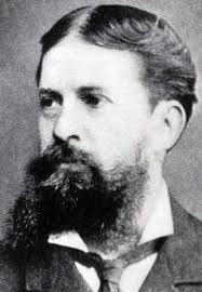
At the start of our seminar, I said that “on weekends this spring (in connection with Phil 6334, but not limited to seminar participants) I will post some of my ‘deconstructions‘ of articles”. I began with Andrew Gelman‘s note “Ethics and the statistical use of prior information”[i], but never posted my deconstruction of it. So since it’s Saturday night, and the seminar is just ending, here it is, along with related links to Stat and ESP research (including me, Jack Good, Persi Diaconis and Pat Suppes). Please share comments especially in relation to current day ESP research. Continue reading
Bayesian/frequentist
Deconstructing Andrew Gelman: “A Bayesian wants everybody else to be a non-Bayesian.”
You can only become coherent by ‘converting’ non-Bayesianly
“What ever happened to Bayesian foundations?” was one of the final topics of our seminar (Mayo/SpanosPhil6334). In the past 15 years or so, not only have (some? most?) Bayesians come to accept violations of the Likelihood Principle, they have also tended to disown Dutch Book arguments, and the very idea of inductive inference as updating beliefs by Bayesian conditionalization has evanescencd. In one of Thursday’s readings, by Baccus, Kyburg, and Thalos (1990)[1], it is argued that under certain conditions, it is never a rational course of action to change belief by Bayesian conditionalization. Here’s a short snippet for your Saturday night reading (the full paper is https://errorstatistics.com/wp-content/uploads/2014/05/bacchus_kyburg_thalos-against-conditionalization.pdf): Continue reading
Phil 6334: Foundations of statistics and its consequences: Day #12
We interspersed key issues from the reading for this session (from Howson and Urbach) with portions of my presentation at the Boston Colloquium (Feb, 2014): Revisiting the Foundations of Statistics in the Era of Big Data: Scaling Up to Meet the Challenge. (Slides below)*.
Someone sent us a recording (mp3)of the panel discussion from that Colloquium (there’s a lot on “big data” and its politics) including: Mayo, Xiao-Li Meng (Harvard), Kent Staley (St. Louis), and Mark van der Laan (Berkeley).
See if this works: | mp3
*There’s a prelude here to our visitor on April 24: Professor Stanley Young from the National Institute of Statistical Sciences.
Phil 6334: Notes on Bayesian Inference: Day #11 Slides
Phil 6334: Duhem’s Problem, highly probable vs highly probed; Day #9 Slides
April 3, 2014: We interspersed discussion with slides; these cover the main readings of the day (check syllabus): the Duhem’s Problem and the Bayesian Way, and “Highly probable vs Highly Probed”. syllabus four. Slides are below (followers of this blog will be familiar with most of this, e.g., here). We also did further work on misspecification testing.
Monday, April 7, is an optional outing, “a seminar class trip”
you might say, here at Thebes at which time we will analyze the statistical curves of the mountains, pie charts of pizza, and (seriously) study some experiments on the problem of replication in “the Hamlet Effect in social psychology”. If you’re around please bop in!
Mayo’s slides on Duhem’s Problem and more from April 3 (Day#9):
Who is allowed to cheat? I.J. Good and that after dinner comedy hour….
It was from my Virginia Tech colleague I.J. Good (in statistics), who died five years ago (April 5, 2009), at 93, that I learned most of what I call “howlers” on this blog. His favorites were based on the “paradoxes” of stopping rules. (I had posted this last year here.)
“In conversation I have emphasized to other statisticians, starting in 1950, that, in virtue of the ‘law of the iterated logarithm,’ by optional stopping an arbitrarily high sigmage, and therefore an arbitrarily small tail-area probability, can be attained even when the null hypothesis is true. In other words if a Fisherian is prepared to use optional stopping (which usually he is not) he can be sure of rejecting a true null hypothesis provided that he is prepared to go on sampling for a long time. The way I usually express this ‘paradox’ is that a Fisherian [but not a Bayesian] can cheat by pretending he has a plane to catch like a gambler who leaves the table when he is ahead” (Good 1983, 135) [*]
Phil 6334: Day #3: Feb 6, 2014
Day #3: Spanos lecture notes 2, and reading/resources from Feb 6 seminar
6334 Day 3 slides: Spanos-lecture-2
___
Crupi & Tentori (2010). Irrelevant Conjunction: Statement and Solution of a New Paradox, Phil Sci, 77, 1–13.
Hawthorne & Fitelson (2004). Re-Solving Irrelevant Conjunction with Probabilistic Independence, Phil Sci 71: 505–514.
Skryms (1975) Choice and Chance 2nd ed. Chapter V and Carnap (pp. 206-211), Dickerson Pub. Co.
Mayo posts on the tacking paradox: Oct. 25, 2013: “Bayesian Confirmation Philosophy and the Tacking Paradox (iv)*” & Oct 25.
An update on this issue will appear shortly in a separate blogpost.
_
READING FOR NEXT WEEK
Selection (pp. 35-59) from: Popper (1962). Conjectures and Refutations: The Growth of Scientific Knowledge. Basic Books.
Objective/subjective, dirty hands and all that: Gelman/ Wasserman blogolog (ii)
Andrew Gelman says that as a philosopher, I should appreciate his blog today in which he records his frustration: “Against aggressive definitions: No, I don’t think it helps to describe Bayes as ‘the analysis of subjective beliefs’…” Gelman writes:
I get frustrated with what might be called “aggressive definitions,” where people use a restrictive definition of something they don’t like. For example, Larry Wasserman writes (as reported by Deborah Mayo):
“I wish people were clearer about what Bayes is/is not and what frequentist inference is/is not. Bayes is the analysis of subjective beliefs but provides no frequency guarantees. Frequentist inference is about making procedures that have frequency guarantees but makes no pretense of representing anyone’s beliefs.”
I’ll accept Larry’s definition of frequentist inference. But as for his definition of Bayesian inference: No no no no no. The probabilities we use in our Bayesian inference are not subjective, or, they’re no more subjective than the logistic regressions and normal distributions and Poisson distributions and so forth that fill up all the textbooks on frequentist inference.
To quickly record some of my own frustrations:*: First, I would disagree with Wasserman’s characterization of frequentist inference, but as is clear from Larry’s comments to (my reaction to him), I think he concurs that he was just giving a broad contrast. Please see Note [1] for a remark from my post: Comments on Wasserman’s “what is Bayesian/frequentist inference?” Also relevant is a Gelman post on the Bayesian name: [2].
Second, Gelman’s “no more subjective than…” evokes remarks I’ve made before. For example, in “What should philosophers of science do…” I wrote:
Arguments given for some very popular slogans (mostly by non-philosophers), are too readily taken on faith as canon by others, and are repeated as gospel. Examples are easily found: all models are false, no models are falsifiable, everything is subjective, or equally subjective and objective, and the only properly epistemological use of probability is to supply posterior probabilities for quantifying actual or rational degrees of belief. Then there is the cluster of “howlers” allegedly committed by frequentist error statistical methods repeated verbatim (discussed on this blog).
I’ve written a lot about objectivity on this blog, e.g., here, here and here (and in real life), but what’s the point if people just rehearse the “everything is a mixture…” line, without making deeply important distinctions? I really think that, next to the “all models are false” slogan, the most confusion has been engendered by the “no methods are objective” slogan. However much we may aim at objective constraints, it is often urged, we can never have “clean hands” free of the influence of beliefs and interests, and we invariably sully methods of inquiry by the entry of background beliefs and personal judgments in their specification and interpretation. Continue reading
Mascots of Bayesneon statistics (rejected post)
(see rejected posts)
U-Phil: Deconstructions [of J. Berger]: Irony & Bad Faith 3
Memory Lane: 2 years ago:
My efficient Errorstat Blogpeople1 have put forward the following 3 reader-contributed interpretive efforts2 as a result of the “deconstruction” exercise from December 11, (mine, from the earlier blog, is at the end) of what I consider:
“….an especially intriguing remark by Jim Berger that I think bears upon the current mindset (Jim is aware of my efforts):
Too often I see people pretending to be subjectivists, and then using “weakly informative” priors that the objective Bayesian community knows are terrible and will give ridiculous answers; subjectivism is then being used as a shield to hide ignorance. . . . In my own more provocative moments, I claim that the only true subjectivists are the objective Bayesians, because they refuse to use subjectivism as a shield against criticism of sloppy pseudo-Bayesian practice. (Berger 2006, 463)” (From blogpost, Dec. 11, 2011)
_________________________________________________
Andrew Gelman:
The statistics literature is big enough that I assume there really is some bad stuff out there that Berger is reacting to, but I think that when he’s talking about weakly informative priors, Berger is not referring to the work in this area that I like, as I think of weakly informative priors as specifically being designed to give answers that are _not_ “ridiculous.”
Keeping things unridiculous is what regularization’s all about, and one challenge of regularization (as compared to pure subjective priors) is that the answer to the question, What is a good regularizing prior?, will depend on the likelihood. There’s a lot of interesting theory and practice relating to weakly informative priors for regularization, a lot out there that goes beyond the idea of noninformativity.
To put it another way: We all know that there’s no such thing as a purely noninformative prior: any model conveys some information. But, more and more, I’m coming across applied problems where I wouldn’t want to be noninformative even if I could, problems where some weak prior information regularizes my inferences and keeps them sane and under control. Continue reading
A. Spanos lecture on “Frequentist Hypothesis Testing”
I attended a lecture by Aris Spanos to his graduate econometrics class here at Va Tech last week[i]. This course, which Spanos teaches every fall, gives a superb illumination of the disparate pieces involved in statistical inference and modeling, and affords clear foundations for how they are linked together. His slides follow the intro section. Some examples with severity assessments are also included.
Frequentist Hypothesis Testing: A Coherent Approach
Aris Spanos
1 Inherent difficulties in learning statistical testing
Statistical testing is arguably the most important, but also the most difficult and confusing chapter of statistical inference for several reasons, including the following.
(i) The need to introduce numerous new notions, concepts and procedures before one can paint — even in broad brushes — a coherent picture of hypothesis testing.
(ii) The current textbook discussion of statistical testing is both highly confusing and confused. There are several sources of confusion.
- (a) Testing is conceptually one of the most sophisticated sub-fields of any scientific discipline.
- (b) Inadequate knowledge by textbook writers who often do not have the technical skills to read and understand the original sources, and have to rely on second hand accounts of previous textbook writers that are often misleading or just outright erroneous. In most of these textbooks hypothesis testing is poorly explained as an idiot’s guide to combining off-the-shelf formulae with statistical tables like the Normal, the Student’s t, the chi-square, etc., where the underlying statistical model that gives rise to the testing procedure is hidden in the background.
- (c) The misleading portrayal of Neyman-Pearson testing as essentially decision-theoretic in nature, when in fact the latter has much greater affinity with the Bayesian rather than the frequentist inference.
- (d) A deliberate attempt to distort and cannibalize frequentist testing by certain Bayesian drumbeaters who revel in (unfairly) maligning frequentist inference in their attempts to motivate their preferred view on statistical inference.
(iii) The discussion of frequentist testing is rather incomplete in so far as it has been beleaguered by serious foundational problems since the 1930s. As a result, different applied fields have generated their own secondary literatures attempting to address these problems, but often making things much worse! Indeed, in some fields like psychology it has reached the stage where one has to correct the ‘corrections’ of those chastising the initial correctors!
In an attempt to alleviate problem (i), the discussion that follows uses a sketchy historical development of frequentist testing. To ameliorate problem (ii), the discussion includes ‘red flag’ pointers (¥) designed to highlight important points that shed light on certain erroneous in- terpretations or misleading arguments. The discussion will pay special attention to (iii), addressing some of the key foundational problems.
[i] It is based on Ch. 14 of Spanos (1999) Probability Theory and Statistical Inference. Cambridge[ii].
[ii] You can win a free copy of this 700+ page text by creating a simple palindrome! https://errorstatistics.com/palindrome/march-contest/
The error statistician has a complex, messy, subtle, ingenious, piece-meal approach
A comment today by Stephen Senn leads me to post the last few sentences of my (2010) paper with David Cox, “Frequentist Statistics as a Theory of Inductive Inference”:
A fundamental tenet of the conception of inductive learning most at home with the frequentist philosophy is that inductive inference requires building up incisive arguments and inferences by putting together several different piece-meal results; we have set out considerations to guide these pieces[i]. Although the complexity of the issues makes it more difficult to set out neatly, as, for example, one could by imagining that a single algorithm encompasses the whole of inductive inference, the payoff is an account that approaches the kind of arguments that scientists build up in order to obtain reliable knowledge and understanding of a field.” (273)[ii]
A reread for Saturday night?
[i]The pieces hang together by dint of the rationale growing out of a severity criterion (or something akin but using a different term.)
[ii]Error and Inference: Recent Exchanges on Experimental Reasoning, Reliability and the Objectivity and Rationality of Science (D Mayo and A. Spanos eds.), Cambridge: Cambridge University Press: 1-27. This paper appeared in The Second Erich L. Lehmann Symposium: Optimality, 2006, Lecture Notes-Monograph Series, Volume 49, Institute of Mathematical Statistics, pp. 247-275.
Stephen Senn: Dawid’s Selection Paradox (guest post)
Stephen Senn
Head, Methodology and Statistics Group,
Competence Center for Methodology and Statistics (CCMS),
Luxembourg
“Dawid’s Selection Paradox”
You can protest, of course, that Dawid’s Selection Paradox is no such thing but then those who believe in the inexorable triumph of logic will deny that anything is a paradox. In a challenging paper published nearly 20 years ago (Dawid 1994), Philip Dawid drew attention to a ‘paradox’ of Bayesian inference. To describe it, I can do no better than to cite the abstract of the paper, which is available from Project Euclid, here: http://projecteuclid.org/DPubS/Repository/1.0/Disseminate?
When the inference to be made is selected after looking at the data, the classical statistical approach demands — as seems intuitively sensible — that allowance be made for the bias thus introduced. From a Bayesian viewpoint, however, no such adjustment is required, even when the Bayesian inference closely mimics the unadjusted classical one. In this paper we examine more closely this seeming inadequacy of the Bayesian approach. In particular, it is argued that conjugate priors for multivariate problems typically embody an unreasonable determinism property, at variance with the above intuition.
I consider this to be an important paper not only for Bayesians but also for frequentists, yet it has only been cited 14 times as of 15 November 2013 according to Google Scholar. In fact I wrote a paper about it in the American Statistician a few years back (Senn 2008) and have also referred to it in a previous blogpost (12 May 2012). That I think it is important and neglected is excuse enough to write about it again.
Philip Dawid is not responsible for my interpretation of his paradox but the way that I understand it can be explained by considering what it means to have a prior distribution. First, as a reminder, if you are going to be 100% Bayesian, which is to say that all of what you will do by way of inference will be to turn a prior into a posterior distribution using the likelihood and the operation of Bayes theorem, then your prior distribution has to satisfy two conditions. First, it must be what you would use to bet now (that is to say at the moment it is established) and second no amount of subsequent data will change your prior qua prior. It will, of course, be updated by Bayes theorem to form a posterior distribution once further data are obtained but that is another matter. The relevant time here is your observation time not the time when the data were collected, so that data that were available in principle but only came to your attention after you established your prior distribution count as further data.
Now suppose that you are going to make an inference about a population mean, θ, using a random sample from the population and choose the standard conjugate prior distribution. Then in that case you will use a Normal distribution with known (to you) parameters μ and σ2. If σ2 is large compared to the random variation you might expect for the means in your sample, then the prior distribution is fairly uninformative and if it is small then fairly informative but being uninformative is not in itself a virtue. Being not informative enough runs the risk that your prior distribution is not one you might wish to use to bet now and being too informative that your prior distribution is one you might be tempted to change given further information. In either of these two cases your prior distribution will be wrong. Thus the task is to be neither too informative nor not informative enough. Continue reading
Highly probable vs highly probed: Bayesian/ error statistical differences
A reader asks: “Can you tell me about disagreements on numbers between a severity assessment within error statistics, and a Bayesian assessment of posterior probabilities?” Sure.
There are differences between Bayesian posterior probabilities and formal error statistical measures, as well as between the latter and a severity (SEV) assessment, which differs from the standard type 1 and 2 error probabilities, p-values, and confidence levels—despite the numerical relationships. Here are some random thoughts that will hopefully be relevant for both types of differences. (Please search this blog for specifics.)
1. The most noteworthy difference is that error statistical inference makes use of outcomes other than the one observed, even after the data are available: there’s no other way to ask things like, how often would you find 1 nominally statistically significant difference in a hunting expedition over k or more factors? Or to distinguish optional stopping with sequential trials from fixed sample size experiments. Here’s a quote I came across just yesterday:
“[S]topping ‘when the data looks good’ can be a serious error when combined with frequentist measures of evidence. For instance, if one used the stopping rule [above]…but analyzed the data as if a fixed sample had been taken, one could guarantee arbitrarily strong frequentist ‘significance’ against H0.” (Berger and Wolpert, 1988, 77).
The worry about being guaranteed to erroneously exclude the true parameter value here is an error statistical affliction that the Bayesian is spared (even though I don’t think they can be too happy about it, especially when HPD intervals are assured of excluding the true parameter value.) See this post for an amusing note; Mayo and Kruse (2001) below; and, if interested, search the (strong) likelihood principle, and Birnbaum.
2. Highly probable vs. highly probed. SEV doesn’t obey the probability calculus: for any test T and outcome x, the severity for both H and ~H might be horribly low. Moreover, an error statistical analysis is not in the business of probabilifying hypotheses but evaluating and controlling the capabilities of methods to discern inferential flaws (problems with linking statistical and scientific claims, problems of interpreting statistical tests and estimates, and problems of underlying model assumptions). This is the basis for applying what may be called the Severity principle. Continue reading
Gelman est effectivement une erreur statistician
A reader calls my attention to Andrew Gelman’s blog announcing a talk that he’s giving today in French: “Philosophie et practique de la statistique bayésienne”. He blogs:
I’ll try to update the slides a bit since a few years ago, to add some thoughts I’ve had recently about problems with noninformative priors, even in simple settings.
The location of the talk will not be convenient for most of you, but anyone who comes to the trouble of showing up will have the opportunity to laugh at my accent.
P.S. For those of you who are interested in the topic but can’t make it to the talk, I recommend these two papers on my non-inductive Bayesian philosophy:
[2013] Philosophy and the practice of Bayesian statistics (with discussion). British Journal of Mathematical and Statistical Psychology, 8–18. (Andrew Gelman and Cosma Shalizi) [2013] Rejoinder to discussion. (Andrew Gelman and Cosma Shalizi)
These papers, especially Gelman (2011), are discussed on this blog (in “U-Phils”). Comments by Senn, Wasserman, and Hennig may be found here, and here,with a response here (please use search for more).
As I say in my comments on Gelman and Shalizi, I think Gelman’s position is (or intends to be) inductive– in the sense of being ampliative (going beyond the data)– but simply not probabilist, i.e., not a matter of updating priors. (A blog post is here)[i]. Here’s a snippet from my comments: Continue reading
“When Bayesian Inference Shatters” Owhadi and Scovel (guest post)
I’m extremely grateful to Drs. Owhadi and Scovel for replying to my request for “a plain Jane” explication of their interesting paper, “When Bayesian Inference Shatters”, and especially for permission to post it. If readers want to ponder the paper awhile and send me comments for guest posts or “U-PHILS*” (by OCT 15), let me know. Feel free to comment as usual in the mean time.
—————————————-
Houman OwhadiProfessor of Applied and Computational Mathematics and Control and Dynamical Systems, Computing + Mathematical Sciences,
California Institute of Technology, USA
“When Bayesian Inference Shatters: A plain Jane explanation”
This is an attempt at a “plain Jane” presentation of the results discussed in the recent arxiv paper “When Bayesian Inference Shatters” located at http://arxiv.org/abs/1308.6306 with the following abstract:
“With the advent of high-performance computing, Bayesian methods are increasingly popular tools for the quantification of uncertainty throughout science and industry. Since these methods impact the making of sometimes critical decisions in increasingly complicated contexts, the sensitivity of their posterior conclusions with respect to the underlying models and prior beliefs is becoming a pressing question. We report new results suggesting that, although Bayesian methods are robust when the number of possible outcomes is finite or when only a finite number of marginals of the data-generating distribution are unknown, they are generically brittle when applied to continuous systems with finite information on the data-generating distribution. This brittleness persists beyond the discretization of continuous systems and suggests that Bayesian inference is generically ill-posed in the sense of Hadamard when applied to such systems: if closeness is defined in terms of the total variation metric or the matching of a finite system of moments, then (1) two practitioners who use arbitrarily close models and observe the same (possibly arbitrarily large amount of) data may reach diametrically opposite conclusions; and (2) any given prior and model can be slightly perturbed to achieve any desired posterior conclusions.”
Now, it is already known from classical Robust Bayesian Inference that Bayesian Inference has some robustness if the random outcomes live in a finite space or if the class of priors considered is finite-dimensional (i.e. what you know is infinite and what you do not know is finite). What we have shown is that if the random outcomes live in an approximation of a continuous space (for instance, when they are decimal numbers given to finite precision) and your class of priors is finite co-dimensional (i.e. what you know is finite and what you do not know may be infinite) then, if the data is observed at a fine enough resolution, the range of posterior values is the deterministic range of the quantity of interest, irrespective of the size of the data. Continue reading
(Part 2) Peircean Induction and the Error-Correcting Thesis
Continuation of “Peircean Induction and the Error-Correcting Thesis”
Deborah G. Mayo
Transactions of the Charles S. Peirce Society: A Quarterly Journal in American Philosophy, Volume 41, Number 2, 2005, pp. 299-319
Part 1 is here.
There are two other points of confusion in critical discussions of the SCT, that we may note here:
I. The SCT and the Requirements of Randomization and Predesignation
The concern with “the trustworthiness of the proceeding” for Peirce like the concern with error probabilities (e.g., significance levels) for error statisticians generally, is directly tied to their view that inductive method should closely link inferences to the methods of data collection as well as to how the hypothesis came to be formulated or chosen for testing.
This account of the rationale of induction is distinguished from others in that it has as its consequences two rules of inductive inference which are very frequently violated (1.95) namely, that the sample be (approximately) random and that the property being tested not be determined by the particular sample x— i.e., predesignation.
The picture of Peircean induction that one finds in critics of the SCT disregards these crucial requirements for induction: Neither enumerative induction nor H-D testing, as ordinarily conceived, requires such rules. Statistical significance testing, however, clearly does.
Suppose, for example that researchers wishing to demonstrate the benefits of HRT search the data for factors on which treated women fare much better than untreated, and finding one such factor they proceed to test the null hypothesis:
H0: there is no improvement in factor F (e.g. memory) among women treated with HRT.
Having selected this factor for testing solely because it is a factor on which treated women show impressive improvement, it is not surprising that this null hypothesis is rejected and the results taken to show a genuine improvement in the population. However, when the null hypothesis is tested on the same data that led it to be chosen for testing, it is well known, a spurious impression of a genuine effect easily results. Suppose, for example, that 20 factors are examined for impressive-looking improvements among HRT-treated women, and the one difference that appears large enough to test turns out to be significant at the 0.05 level. The actual significance level—the actual probability of reporting a statistically significant effect when in fact the null hypothesis is true—is not 5% but approximately 64% (Mayo 1996, Mayo and Kruse 2001, Mayo and Cox 2006). To infer the denial of H0, and infer there is evidence that HRT improves memory, is to make an inference with low severity (approximately 0.36).
II Understanding the “long-run error correcting” metaphor
Discussions of Peircean ‘self-correction’ often confuse two interpretations of the ‘long-run’ error correcting metaphor, even in the case of quantitative induction: (a) Asymptotic self-correction (as n approaches ∞): In this construal, it is imagined that one has a sample, say of size n=10, and it is supposed that the SCT assures us that as the sample size increases toward infinity, one gets better and better estimates of some feature of the population, say the mean. Although this may be true, provided assumptions of a statistical model (e.g., the Binomial) are met, it is not the sense intended in significance-test reasoning nor, I maintain, in Peirce’s SCT. Peirce’s idea, instead, gives needed insight for understanding the relevance of ‘long-run’ error probabilities of significance tests to assess the reliability of an inductive inference from a specific set of data, (b) Error probabilities of a test: In this construal, one has a sample of size n, say 10, and imagines hypothetical replications of the experiment—each with samples of 10. Each sample of 10 gives a single value of the test statistic d(X), but one can consider the distribution of values that would occur in hypothetical repetitions (of the given type of sampling). The probability distribution of d(X) is called the sampling distribution, and the correct calculation of the significance level is an example of how tests appeal to this distribution: Thanks to the relationship between the observed d(x) and the sampling distribution of d(X), the former can be used to reliably probe the correctness of statistical hypotheses (about the procedure) that generated the particular 10-fold sample. That is what the SCT is asserting.
It may help to consider a very informal example. Suppose that weight gain is measured by 10 well-calibrated and stable methods, possibly using several measuring instruments and the results show negligible change over a test period of interest. This may be regarded as grounds for inferring that the individual’s weight gain is negligible within limits set by the sensitivity of the scales. Why? While it is true that by averaging more and more weight measurements, i.e., an eleventh, twelfth, etc., one would get asymptotically close to the true weight, that is not the rationale for the particular inference. The rationale is rather that the error probabilistic properties of the weighing procedure (the probability of ten-fold weighings erroneously failing to show weight change) inform one of the correct weight in the case at hand, e.g., that a 0 observed weight increase passes the “no-weight gain” hypothesis with high severity. Continue reading
Peircean Induction and the Error-Correcting Thesis (Part I)
Today is C.S. Peirce’s birthday. I hadn’t blogged him before, but he’s one of my all time heroes. You should read him: he’s a treasure chest on essentially any topic. I’ll blog the main sections of a (2005) paper over the next few days. It’s written for a very general philosophical audience; the statistical parts are pretty informal. Happy birthday Peirce.
Peircean Induction and the Error-Correcting Thesis
Deborah G. Mayo
Transactions of the Charles S. Peirce Society: A Quarterly Journal in American Philosophy, Volume 41, Number 2, 2005, pp. 299-319
Peirce’s philosophy of inductive inference in science is based on the idea that what permits us to make progress in science, what allows our knowledge to grow, is the fact that science uses methods that are self-correcting or error-correcting:
Induction is the experimental testing of a theory. The justification of it is that, although the conclusion at any stage of the investigation may be more or less erroneous, yet the further application of the same method must correct the error. (5.145)
Inductive methods—understood as methods of experimental testing—are justified to the extent that they are error-correcting methods. We may call this Peirce’s error-correcting or self-correcting thesis (SCT):
Self-Correcting Thesis SCT: methods for inductive inference in science are error correcting; the justification for inductive methods of experimental testing in science is that they are self-correcting.
Peirce’s SCT has been a source of fascination and frustration. By and large, critics and followers alike have denied that Peirce can sustain his SCT as a way to justify scientific induction: “No part of Peirce’s philosophy of science has been more severely criticized, even by his most sympathetic commentators, than this attempted validation of inductive methodology on the basis of its purported self-correctiveness” (Rescher 1978, p. 20).
In this paper I shall revisit the Peircean SCT: properly interpreted, I will argue, Peirce’s SCT not only serves its intended purpose, it also provides the basis for justifying (frequentist) statistical methods in science. While on the one hand, contemporary statistical methods increase the mathematical rigor and generality of Peirce’s SCT, on the other, Peirce provides something current statistical methodology lacks: an account of inductive inference and a philosophy of experiment that links the justification for statistical tests to a more general rationale for scientific induction. Combining the mathematical contributions of modern statistics with the inductive philosophy of Peirce, sets the stage for developing an adequate justification for contemporary inductive statistical methodology.
2. Probabilities are assigned to procedures not hypotheses
Peirce’s philosophy of experimental testing shares a number of key features with the contemporary (Neyman and Pearson) Statistical Theory: statistical methods provide, not means for assigning degrees of probability, evidential support, or confirmation to hypotheses, but procedures for testing (and estimation), whose rationale is their predesignated high frequencies of leading to correct results in some hypothetical long-run. A Neyman and Pearson (NP) statistical test, for example, instructs us “To decide whether a hypothesis, H, of a given type be rejected or not, calculate a specified character, x0, of the observed facts; if x> x0 reject H; if x< x0 accept H.” Although the outputs of N-P tests do not assign hypotheses degrees of probability, “it may often be proved that if we behave according to such a rule … we shall reject H when it is true not more, say, than once in a hundred times, and in addition we may have evidence that we shall reject H sufficiently often when it is false” (Neyman and Pearson, 1933, p.142).[i]
The relative frequencies of erroneous rejections and erroneous acceptances in an actual or hypothetical long run sequence of applications of tests are error probabilities; we may call the statistical tools based on error probabilities, error statistical tools. In describing his theory of inference, Peirce could be describing that of the error-statistician:
The theory here proposed does not assign any probability to the inductive or hypothetic conclusion, in the sense of undertaking to say how frequently that conclusion would be found true. It does not propose to look through all the possible universes, and say in what proportion of them a certain uniformity occurs; such a proceeding, were it possible, would be quite idle. The theory here presented only says how frequently, in this universe, the special form of induction or hypothesis would lead us right. The probability given by this theory is in every way different—in meaning, numerical value, and form—from that of those who would apply to ampliative inference the doctrine of inverse chances. (2.748)
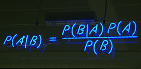
The doctrine of “inverse chances” alludes to assigning (posterior) probabilities in hypotheses by applying the definition of conditional probability (Bayes’s theorem)—a computation requires starting out with a (prior or “antecedent”) probability assignment to an exhaustive set of hypotheses:
If these antecedent probabilities were solid statistical facts, like those upon which the insurance business rests, the ordinary precepts and practice [of inverse probability] would be sound. But they are not and cannot be statistical facts. What is the antecedent probability that matter should be composed of atoms? Can we take statistics of a multitude of different universes? (2.777)
For Peircean induction, as in the N-P testing model, the conclusion or inference concerns a hypothesis that either is or is not true in this one universe; thus, assigning a frequentist probability to a particular conclusion, other than the trivial ones of 1 or 0, for Peirce, makes sense only “if universes were as plentiful as blackberries” (2.684). Thus the Bayesian inverse probability calculation seems forced to rely on subjective probabilities for computing inverse inferences, but “subjective probabilities” Peirce charges “express nothing but the conformity of a new suggestion to our prepossessions, and these are the source of most of the errors into which man falls, and of all the worse of them” (2.777).
Hearing Pierce contrast his view of induction with the more popular Bayesian account of his day (the Conceptualists), one could be listening to an error statistician arguing against the contemporary Bayesian (subjective or other)—with one important difference. Today’s error statistician seems to grant too readily that the only justification for N-P test rules is their ability to ensure we will rarely take erroneous actions with respect to hypotheses in the long run of applications. This so called inductive behavior rationale seems to supply no adequate answer to the question of what is learned in any particular application about the process underlying the data. Peirce, by contrast, was very clear that what is really wanted in inductive inference in science is the ability to control error probabilities of test procedures, i.e., “the trustworthiness of the proceeding”. Moreover it is only by a faulty analogy with deductive inference, Peirce explains, that many suppose that inductive (synthetic) inference should supply a probability to the conclusion: “… in the case of analytic inference we know the probability of our conclusion (if the premises are true), but in the case of synthetic inferences we only know the degree of trustworthiness of our proceeding (“The Probability of Induction” 2.693).
Knowing the “trustworthiness of our inductive proceeding”, I will argue, enables determining the test’s probative capacity, how reliably it detects errors, and the severity of the test a hypothesis withstands. Deliberately making use of known flaws and fallacies in reasoning with limited and uncertain data, tests may be constructed that are highly trustworthy probes in detecting and discriminating errors in particular cases. This, in turn, enables inferring which inferences about the process giving rise to the data are and are not warranted: an inductive inference to hypothesis H is warranted to the extent that with high probability the test would have detected a specific flaw or departure from what H asserts, and yet it did not.
3. So why is justifying Peirce’s SCT thought to be so problematic?
You can read Section 3 here. (it’s not necessary for understanding the rest).
4. Peircean induction as severe testing
… [I]nduction, for Peirce, is a matter of subjecting hypotheses to “the test of experiment” (7.182).
The process of testing it will consist, not in examining the facts, in order to see how well they accord with the hypothesis, but on the contrary in examining such of the probable consequences of the hypothesis … which would be very unlikely or surprising in case the hypothesis were not true. (7.231)
When, however, we find that prediction after prediction, notwithstanding a preference for putting the most unlikely ones to the test, is verified by experiment,…we begin to accord to the hypothesis a standing among scientific results.
This sort of inference it is, from experiments testing predictions based on a hypothesis, that is alone properly entitled to be called induction. (7.206)
While these and other passages are redolent of Popper, Peirce differs from Popper in crucial ways. Peirce, unlike Popper, is primarily interested not in falsifying claims but in the positive pieces of information provided by tests, with “the corrections called for by the experiment” and with the hypotheses, modified or not, that manage to pass severe tests. For Popper, even if a hypothesis is highly corroborated (by his lights), he regards this as at most a report of the hypothesis’ past performance and denies it affords positive evidence for its correctness or reliability. Further, Popper denies that he could vouch for the reliability of the method he recommends as “most rational”—conjecture and refutation. Indeed, Popper’s requirements for a highly corroborated hypothesis are not sufficient for ensuring severity in Peirce’s sense (Mayo 1996, 2003, 2005). Where Popper recoils from even speaking of warranted inductions, Peirce conceives of a proper inductive inference as what had passed a severe test—one which would, with high probability, have detected an error if present.
In Peirce’s inductive philosophy, we have evidence for inductively inferring a claim or hypothesis H when not only does H “accord with” the data x; but also, so good an accordance would very probably not have resulted, were H not true. In other words, we may inductively infer H when it has withstood a test of experiment that it would not have withstood, or withstood so well, were H not true (or were a specific flaw present). This can be encapsulated in the following severity requirement for an experimental test procedure, ET, and data set x.
Hypothesis H passes a severe test with x iff (firstly) x accords with H and (secondly) the experimental test procedure ET would, with very high probability, have signaled the presence of an error were there a discordancy between what H asserts and what is correct (i.e., were H false).
The test would “have signaled an error” by having produced results less accordant with H than what the test yielded. Thus, we may inductively infer H when (and only when) H has withstood a test with high error detecting capacity, the higher this probative capacity, the more severely H has passed. What is assessed (quantitatively or qualitatively) is not the amount of support for H but the probative capacity of the test of experiment ET (with regard to those errors that an inference to H is declaring to be absent)……….
You can read the rest of Section 4 here.
5. The path from qualitative to quantitative induction
In my understanding of Peircean induction, the difference between qualitative and quantitative induction is really a matter of degree, according to whether their trustworthiness or severity is quantitatively or only qualitatively ascertainable. This reading not only neatly organizes Peirce’s typologies of the various types of induction, it underwrites the manner in which, within a given classification, Peirce further subdivides inductions by their “strength”.
(I) First-Order, Rudimentary or Crude Induction
Consider Peirce’s First Order of induction: the lowest, most rudimentary form that he dubs, the “pooh-pooh argument”. It is essentially an argument from ignorance: Lacking evidence for the falsity of some hypothesis or claim H, provisionally adopt H. In this very weakest sort of induction, crude induction, the most that can be said is that a hypothesis would eventually be falsified if false. (It may correct itself—but with a bang!) It “is as weak an inference as any that I would not positively condemn” (8.237). While uneliminable in ordinary life, Peirce denies that rudimentary induction is to be included as scientific induction. Without some reason to think evidence of H‘s falsity would probably have been detected, were H false, finding no evidence against H is poor inductive evidence for H. H has passed only a highly unreliable error probe. Continue reading
Bad news bears: ‘Bayesian bear’ rejoinder-reblog mashup
Oh No! It’s those mutant bears again. To my dismay, I’ve been sent, for the third time, that silly, snarky, adolescent, clip of those naughty “what the p-value” bears (first posted on Aug 5, 2012), who cannot seem to get a proper understanding of significance tests into their little bear brains. So apparently some people haven’t seen my rejoinder which, as I said then, practically wrote itself. So since it’s Saturday night here at the Elbar Room, let’s listen in to a mashup of both the clip and my original rejoinder (in which p-value bears are replaced with hypothetical Bayesian bears).
These stilted bear figures and their voices are sufficiently obnoxious in their own right, even without the tedious lampooning of p-values and the feigned horror at learning they should not be reported as posterior probabilities.
Mayo’s Rejoinder:
Bear #1: Do you have the results of the study?
Bear #2:Yes. The good news is there is a .996 probability of a positive difference in the main comparison.
Bear #1: Great. So I can be well assured that there is just a .004 probability that such positive results would occur if they were merely due to chance.
Bear #2: Not really, that would be an incorrect interpretation. Continue reading
Why I am not a “dualist” in the sense of Sander Greenland
This post picks up, and continues, an exchange that began with comments on my June 14 blogpost (between Sander Greenland, Nicole Jinn, and I). My new response is at the end. The concern is how to expose and ideally avoid some of the well known flaws and foibles in statistical inference, thanks to gaps between data and statistical inference, and between statistical inference and substantive claims. I am not rejecting the use of multiple methods in the least (they are highly valuable when one method is capable of detecting or reducing flaws in one or more others). Nor am I speaking of classical dualism in metaphysics (which I also do not espouse). I begin with Greenland’s introduction of this idea in his comment… (For various earlier comments, see the post.)
…. I sense some confusion of criticism of the value of tests as popular tools vs. criticism of their logical foundation. I am a critic in the first, practical category, who regards the adoption of testing outside of narrow experimental programs as an unmitigated disaster, resulting in publication bias, prosecutor-type fallacies, and affirming the consequent fallacies throughout the health and social science literature. Even though testing can in theory be used soundly, it just hasn’t done well in practice in these fields. This could be ascribed to human failings rather than failings of received testing theories, but I would require any theory of applied statistics to deal with human limitations, just as safety engineering must do for physical products. I regard statistics as having been woefully negligent of cognitive psychology in this regard. In particular, widespread adoption and vigorous defense of a statistical method or philosophy is no more evidence of its scientific value than widespread adoption and vigorous defense of a religion is evidence of its scientific value. That should bring us to alternatives. I am aware of no compelling data showing that other approaches would have done better, but I do find compelling the arguments that at least some of the problems would have been mitigated by teaching a dualist approach to statistics, in which every procedure must be supplied with both an accurate frequentist and an accurate Bayesian interpretation, if only to reduce prevalent idiocies like interpreting a two-sided P-value as “the” posterior probability of a point null hypothesis.
Nicole Jinn (to Sander Greenland)
What exactly is this ‘dualist’ approach to teaching statistics and why does it mitigate the problems, as you claim? (I am increasingly interested in finding more effective ways to teach/instruct others in various age groups about statistics.) I have a difficult time seeing how effective this ‘dualist’ way of teaching could be for the following reason: the Bayesian and frequentist approaches are vastly different in their aims and the way they see statistics being used in (natural or social) science, especially when one looks more carefully at the foundations of each methodology (e.g., disagreements about where exactly probability enters into inference, or about what counts as relevant information). Hence, it does not make sense (to me) to supply both types of interpretation to the same data and the same research question! Instead, it makes more sense (from a teaching perspective) to demonstrate a Bayesian interpretation for one experiment, and a frequentist interpretation for another experiment, in the hopes of getting at the (major) differences between the two methodologies.
Sander. Thanks for your comment. Interestingly, I think the conglomeration of error statistical tools are the ones most apt at dealing with human limitations and foibles: they give piecemeal methods to ask one question at a time (e.g., would we be mistaken to suppose there is evidence of any effect at all? mistaken about how large? about iid assumptions? about possible causes? about implications for distinguishing any theories?). The standard Bayesian apparatus requires setting out a complete set of hypotheses that might arise, plus prior probabilities in each of them (or in “catchall” hypotheses), as well as priors in the model…and after this herculean task is complete, there is a purely deductive update: being deductive it never goes beyond the givens. Perhaps the data will require a change in your prior—this is what you must have believed before, since otherwise you find your posterior unacceptable—thereby encouraging the very self-sealing inferences we all claim to deplore. Continue reading


